Location
Location ANSS
The ANSS event ID is ak020ec8mji8 and the event page is at
https://earthquake.usgs.gov/earthquakes/eventpage/ak020ec8mji8/executive.
2020/11/07 15:03:54 61.517 -149.917 43.7 4.4 Alaska
Focal Mechanism
 USGS/SLU Moment Tensor Solution
 ENS  2020/11/07 15:03:54:0  61.52 -149.92  43.7 4.4 Alaska

 Stations used:
   AK.BMR AK.CAPN AK.CAST AK.CCB AK.DHY AK.DIV AK.DOT AK.EYAK
   AK.FID AK.FIRE AK.GHO AK.GLB AK.GLI AK.HIN AK.J19K AK.J25K
   AK.KLU AK.KNK AK.KTH AK.L19K AK.L20K AK.M20K AK.M26K
   AK.N18K AK.N19K AK.O19K AK.P23K AK.PAX AK.PPLA AK.PWL
   AK.Q23K AK.RC01 AK.RIDG AK.SAW AK.SCM AK.SKN AK.SLK AK.SSN
   AK.SWD AK.TGL AK.TRF AT.MENT AT.PMR AV.ILSW AV.RED AV.SPU
   AV.STLK TA.J18K TA.M22K TA.O22K

 Filtering commands used:
   cut o DIST/3.3 -40 o DIST/3.3 +50
   rtr
   taper w 0.1
   hp c 0.03 n 3
   lp c 0.08 n 3

 Best Fitting Double Couple
  Mo = 4.22e+22 dyne-cm
  Mw = 4.35
  Z  = 51 km
  Plane   Strike  Dip  Rake
   NP1      200    60   -65
   NP2      337    38   -126
  Principal Axes:
   Axis    Value   Plunge  Azimuth
    T   4.22e+22     12     272
    N   0.00e+00     21       7
    P  -4.22e+22     65     156

 Moment Tensor: (dyne-cm)
    Component   Value
       Mxx    -6.05e+21
       Mxy     1.19e+21
       Mxz     1.49e+22
       Myy     3.91e+22
       Myz    -1.49e+22
       Mzz    -3.31e+22


                     --------------
                 ###########---########
              ###############--###########
             ##############------##########
           ###############---------##########
          ###############------------#########
         ##############---------------#########
        ###############----------------#########
        ##############------------------########
       #   ##########--------------------########
       # T #########---------------------########
       #   #########---------------------########
       ############-----------------------#######
        ###########----------   ----------######
        ###########---------- P ----------######
         ##########----------   ----------#####
          #########----------------------#####
           ########----------------------####
             ######---------------------###
              #####--------------------###
                 ###------------------#
                     --------------


 Global CMT Convention Moment Tensor:
      R          T          P
 -3.31e+22   1.49e+22   1.49e+22
  1.49e+22  -6.05e+21  -1.19e+21
  1.49e+22  -1.19e+21   3.91e+22


Details of the solution is found at

http://www.eas.slu.edu/eqc/eqc_mt/MECH.NA/20201107150354/index.html
|
Preferred Solution
The preferred solution from an analysis of the surface-wave spectral amplitude radiation pattern, waveform inversion or first motion observations is
      STK = 200
      DIP = 60
     RAKE = -65
       MW = 4.35
       HS = 51.0
The NDK file is 20201107150354.ndk
The waveform inversion is preferred.
Moment Tensor Comparison
The following compares this source inversion to those provided by others. The purpose is to look for major differences and also to note slight differences that might be inherent to the processing procedure. For completeness the USGS/SLU solution is repeated from above.
| SLU |
USGSMWR |
 USGS/SLU Moment Tensor Solution
 ENS  2020/11/07 15:03:54:0  61.52 -149.92  43.7 4.4 Alaska

 Stations used:
   AK.BMR AK.CAPN AK.CAST AK.CCB AK.DHY AK.DIV AK.DOT AK.EYAK
   AK.FID AK.FIRE AK.GHO AK.GLB AK.GLI AK.HIN AK.J19K AK.J25K
   AK.KLU AK.KNK AK.KTH AK.L19K AK.L20K AK.M20K AK.M26K
   AK.N18K AK.N19K AK.O19K AK.P23K AK.PAX AK.PPLA AK.PWL
   AK.Q23K AK.RC01 AK.RIDG AK.SAW AK.SCM AK.SKN AK.SLK AK.SSN
   AK.SWD AK.TGL AK.TRF AT.MENT AT.PMR AV.ILSW AV.RED AV.SPU
   AV.STLK TA.J18K TA.M22K TA.O22K

 Filtering commands used:
   cut o DIST/3.3 -40 o DIST/3.3 +50
   rtr
   taper w 0.1
   hp c 0.03 n 3
   lp c 0.08 n 3

 Best Fitting Double Couple
  Mo = 4.22e+22 dyne-cm
  Mw = 4.35
  Z  = 51 km
  Plane   Strike  Dip  Rake
   NP1      200    60   -65
   NP2      337    38   -126
  Principal Axes:
   Axis    Value   Plunge  Azimuth
    T   4.22e+22     12     272
    N   0.00e+00     21       7
    P  -4.22e+22     65     156

 Moment Tensor: (dyne-cm)
    Component   Value
       Mxx    -6.05e+21
       Mxy     1.19e+21
       Mxz     1.49e+22
       Myy     3.91e+22
       Myz    -1.49e+22
       Mzz    -3.31e+22


                     --------------
                 ###########---########
              ###############--###########
             ##############------##########
           ###############---------##########
          ###############------------#########
         ##############---------------#########
        ###############----------------#########
        ##############------------------########
       #   ##########--------------------########
       # T #########---------------------########
       #   #########---------------------########
       ############-----------------------#######
        ###########----------   ----------######
        ###########---------- P ----------######
         ##########----------   ----------#####
          #########----------------------#####
           ########----------------------####
             ######---------------------###
              #####--------------------###
                 ###------------------#
                     --------------


 Global CMT Convention Moment Tensor:
      R          T          P
 -3.31e+22   1.49e+22   1.49e+22
  1.49e+22  -6.05e+21  -1.19e+21
  1.49e+22  -1.19e+21   3.91e+22


Details of the solution is found at

http://www.eas.slu.edu/eqc/eqc_mt/MECH.NA/20201107150354/index.html
|
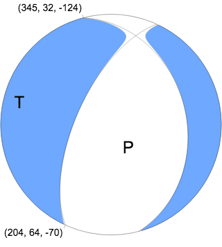
Regional Moment Tensor (Mwr)
Moment 4.580e+15 N-m
Magnitude 4.37 Mwr
Depth 52.0 km
Percent DC 98%
Half Duration -
Catalog US
Data Source US 3
Contributor US 3

Nodal Planes
Plane Strike Dip Rake
NP1 345 32 -124
NP2 204 64 -70

Principal Axes
Axis Value Plunge Azimuth
T 4.606e+15 N-m 17 280
N -0.052e+15 N-m 17 16
P -4.554e+15 N-m 65 149
|
Magnitudes
Given the availability of digital waveforms for determination of the moment tensor, this section documents the added processing leading to mLg, if appropriate to the region, and ML by application of the respective IASPEI formulae. As a research study, the linear distance term of the IASPEI formula
for ML is adjusted to remove a linear distance trend in residuals to give a regionally defined ML. The defined ML uses horizontal component recordings, but the same procedure is applied to the vertical components since there may be some interest in vertical component ground motions. Residual plots versus distance may indicate interesting features of ground motion scaling in some distance ranges. A residual plot of the regionalized magnitude is given as a function of distance and azimuth, since data sets may transcend different wave propagation provinces.
ML Magnitude
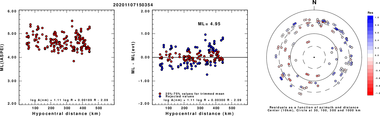
Left: ML computed using the IASPEI formula for Horizontal components. Center: ML residuals computed using a modified IASPEI formula that accounts for path specific attenuation; the values used for the trimmed mean are indicated. The ML relation used for each figure is given at the bottom of each plot.
Right: Residuals from new relation as a function of distance and azimuth.
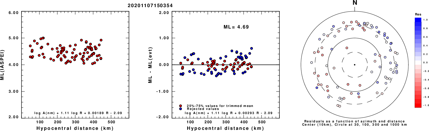
Left: ML computed using the IASPEI formula for Vertical components (research). Center: ML residuals computed using a modified IASPEI formula that accounts for path specific attenuation; the values used for the trimmed mean are indicated. The ML relation used for each figure is given at the bottom of each plot.
Right: Residuals from new relation as a function of distance and azimuth.
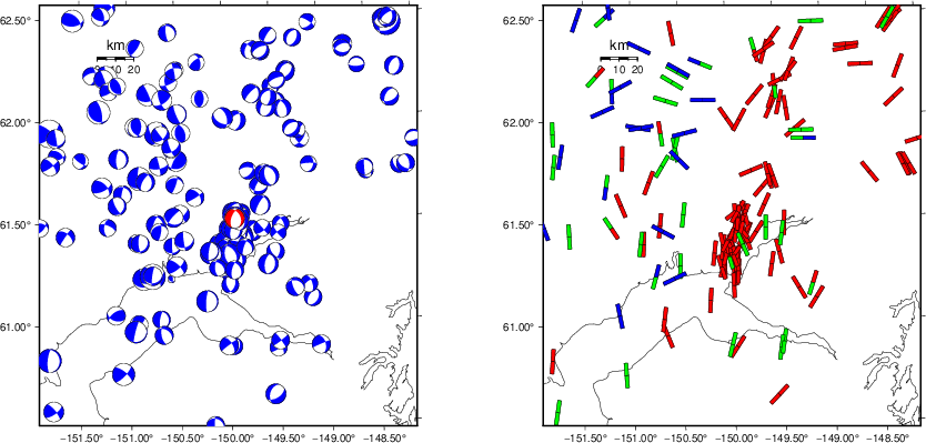
Context
The left panel of the next figure presents the focal mechanism for this earthquake (red) in the context of other nearby events (blue) in the SLU Moment Tensor Catalog. The right panel shows the inferred direction of maximum compressive stress and the type of faulting (green is strike-slip, red is normal, blue is thrust; oblique is shown by a combination of colors). Thus context plot is useful for assessing the appropriateness of the moment tensor of this event.
Waveform Inversion using wvfgrd96
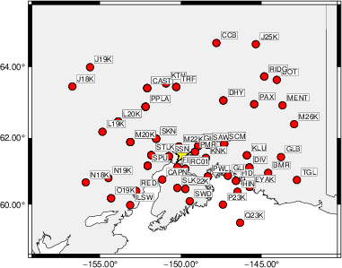
The focal mechanism was determined using broadband seismic waveforms. The location of the event (star) and the
stations used for (red) the waveform inversion are shown in the next figure.
|
|
Location of broadband stations used for waveform inversion
|
The program wvfgrd96 was used with good traces observed at short distance to determine the focal mechanism, depth and seismic moment. This technique requires a high quality signal and well determined velocity model for the Green's functions. To the extent that these are the quality data, this type of mechanism should be preferred over the radiation pattern technique which requires the separate step of defining the pressure and tension quadrants and the correct strike.
The observed and predicted traces are filtered using the following gsac commands:
cut o DIST/3.3 -40 o DIST/3.3 +50
rtr
taper w 0.1
hp c 0.03 n 3
lp c 0.08 n 3
The results of this grid search are as follow:
           DEPTH  STK   DIP  RAKE   MW    FIT
WVFGRD96    1.0   185    45    90   3.53 0.2016
WVFGRD96    2.0   185    45    90   3.67 0.2607
WVFGRD96    3.0   175    50    75   3.72 0.2404
WVFGRD96    4.0   140    90   -45   3.69 0.2265
WVFGRD96    5.0   135    80   -45   3.72 0.2461
WVFGRD96    6.0   135    75   -40   3.74 0.2620
WVFGRD96    7.0   135    75   -40   3.76 0.2768
WVFGRD96    8.0   130    65   -35   3.81 0.2809
WVFGRD96    9.0   130    65   -40   3.83 0.2904
WVFGRD96   10.0    70    45    35   3.84 0.2992
WVFGRD96   11.0    70    45    35   3.85 0.3090
WVFGRD96   12.0    70    50    35   3.87 0.3191
WVFGRD96   13.0    70    50    35   3.88 0.3279
WVFGRD96   14.0    70    50    35   3.89 0.3349
WVFGRD96   15.0    70    55    35   3.91 0.3414
WVFGRD96   16.0    70    55    35   3.92 0.3474
WVFGRD96   17.0    70    55    35   3.93 0.3527
WVFGRD96   18.0    70    55    35   3.94 0.3576
WVFGRD96   19.0    70    55    35   3.95 0.3619
WVFGRD96   20.0    70    60    40   3.97 0.3668
WVFGRD96   21.0    70    60    40   3.99 0.3705
WVFGRD96   22.0    70    60    40   4.00 0.3745
WVFGRD96   23.0    70    60    40   4.01 0.3778
WVFGRD96   24.0    70    60    40   4.02 0.3798
WVFGRD96   25.0    65    65    40   4.03 0.3811
WVFGRD96   26.0   225    60   -30   4.02 0.3874
WVFGRD96   27.0   225    65   -35   4.03 0.3952
WVFGRD96   28.0   225    65   -35   4.05 0.4045
WVFGRD96   29.0   220    60   -40   4.05 0.4132
WVFGRD96   30.0   220    60   -40   4.07 0.4227
WVFGRD96   31.0   220    65   -40   4.08 0.4326
WVFGRD96   32.0   220    65   -40   4.09 0.4421
WVFGRD96   33.0   220    65   -40   4.10 0.4498
WVFGRD96   34.0   220    65   -40   4.11 0.4583
WVFGRD96   35.0   215    70   -50   4.11 0.4705
WVFGRD96   36.0   215    70   -50   4.13 0.4858
WVFGRD96   37.0   215    70   -50   4.14 0.4997
WVFGRD96   38.0   210    65   -55   4.15 0.5123
WVFGRD96   39.0   210    65   -50   4.17 0.5278
WVFGRD96   40.0   210    65   -60   4.26 0.5430
WVFGRD96   41.0   205    65   -65   4.27 0.5544
WVFGRD96   42.0   205    60   -65   4.28 0.5647
WVFGRD96   43.0   205    60   -65   4.29 0.5743
WVFGRD96   44.0   205    60   -65   4.30 0.5823
WVFGRD96   45.0   205    60   -65   4.31 0.5896
WVFGRD96   46.0   200    60   -65   4.32 0.5954
WVFGRD96   47.0   200    60   -65   4.33 0.6012
WVFGRD96   48.0   200    60   -65   4.34 0.6046
WVFGRD96   49.0   200    60   -65   4.34 0.6081
WVFGRD96   50.0   200    60   -65   4.35 0.6099
WVFGRD96   51.0   200    60   -65   4.35 0.6110
WVFGRD96   52.0   200    60   -65   4.36 0.6105
WVFGRD96   53.0   200    60   -65   4.36 0.6093
WVFGRD96   54.0   200    60   -65   4.37 0.6073
WVFGRD96   55.0   200    60   -65   4.37 0.6040
WVFGRD96   56.0   200    60   -65   4.37 0.6008
WVFGRD96   57.0   200    60   -65   4.37 0.5960
WVFGRD96   58.0   200    60   -65   4.37 0.5916
WVFGRD96   59.0   200    60   -65   4.38 0.5864
The best solution is
WVFGRD96 51.0 200 60 -65 4.35 0.6110
The mechanism corresponding to the best fit is
|
|
Figure 1. Waveform inversion focal mechanism
|
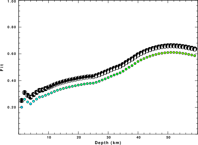
The best fit as a function of depth is given in the following figure:
|
|
Figure 2. Depth sensitivity for waveform mechanism
|
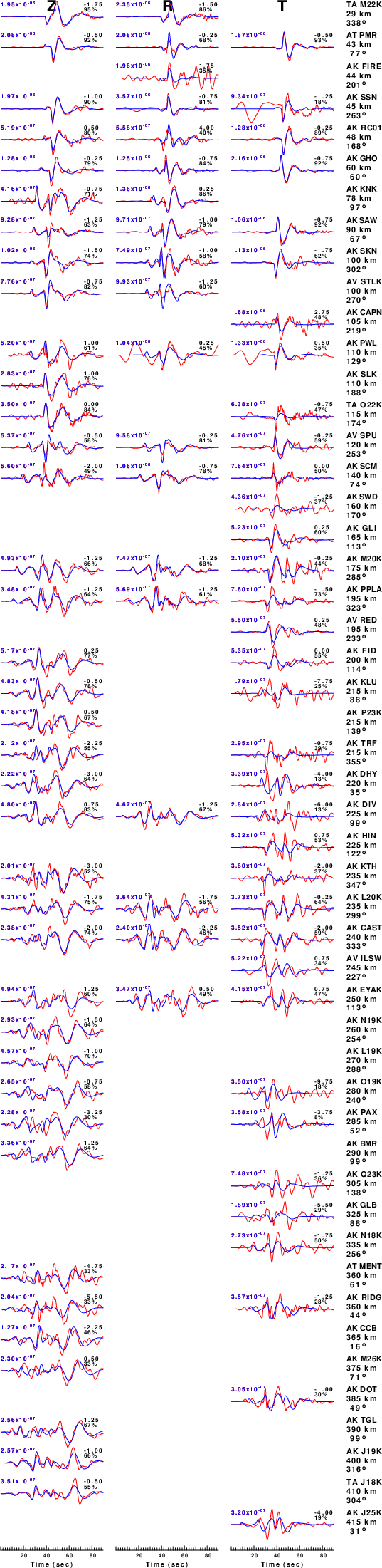
The comparison of the observed and predicted waveforms is given in the next figure. The red traces are the observed and the blue are the predicted.
Each observed-predicted component is plotted to the same scale and peak amplitudes are indicated by the numbers to the left of each trace. A pair of numbers is given in black at the right of each predicted traces. The upper number it the time shift required for maximum correlation between the observed and predicted traces. This time shift is required because the synthetics are not computed at exactly the same distance as the observed, the velocity model used in the predictions may not be perfect and the epicentral parameters may be be off.
A positive time shift indicates that the prediction is too fast and should be delayed to match the observed trace (shift to the right in this figure). A negative value indicates that the prediction is too slow. The lower number gives the percentage of variance reduction to characterize the individual goodness of fit (100% indicates a perfect fit).
The bandpass filter used in the processing and for the display was
cut o DIST/3.3 -40 o DIST/3.3 +50
rtr
taper w 0.1
hp c 0.03 n 3
lp c 0.08 n 3
|
|
Figure 3. Waveform comparison for selected depth. Red: observed; Blue - predicted. The time shift with respect to the model prediction is indicated. The percent of fit is also indicated. The time scale is relative to the first trace sample.
|
|
|
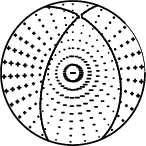
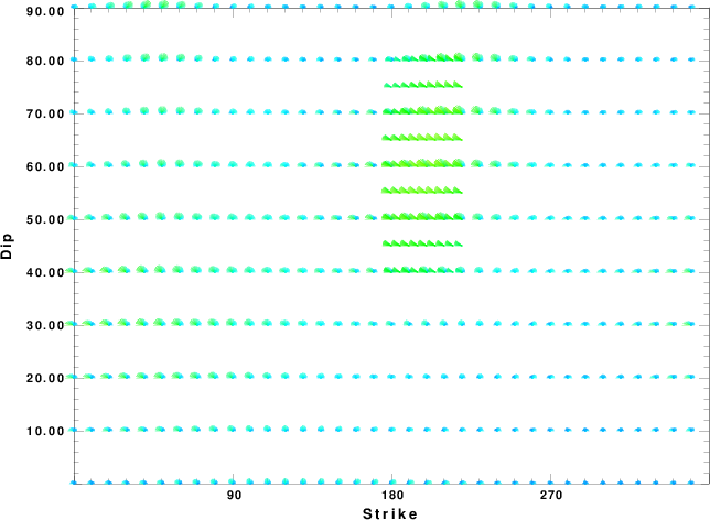
Focal mechanism sensitivity at the preferred depth. The red color indicates a very good fit to the waveforms.
Each solution is plotted as a vector at a given value of strike and dip with the angle of the vector representing the rake angle, measured, with respect to the upward vertical (N) in the figure.
|
A check on the assumed source location is possible by looking at the time shifts between the observed and predicted traces. The time shifts for waveform matching arise for several reasons:
- The origin time and epicentral distance are incorrect
- The velocity model used for the inversion is incorrect
- The velocity model used to define the P-arrival time is not the
same as the velocity model used for the waveform inversion
(assuming that the initial trace alignment is based on the
P arrival time)
Assuming only a mislocation, the time shifts are fit to a functional form:
Time_shift = A + B cos Azimuth + C Sin Azimuth
The time shifts for this inversion lead to the next figure:
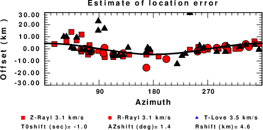
The derived shift in origin time and epicentral coordinates are given at the bottom of the figure.
Velocity Model
The WUS.model used for the waveform synthetic seismograms and for the surface wave eigenfunctions and dispersion is as follows
(The format is in the model96 format of Computer Programs in Seismology).
MODEL.01
Model after     8 iterations
ISOTROPIC
KGS
FLAT EARTH
1-D
CONSTANT VELOCITY
LINE08
LINE09
LINE10
LINE11
      H(KM)   VP(KM/S)   VS(KM/S) RHO(GM/CC)         QP         QS       ETAP       ETAS      FREFP      FREFS
     1.9000     3.4065     2.0089     2.2150  0.302E-02  0.679E-02   0.00       0.00       1.00       1.00
     6.1000     5.5445     3.2953     2.6089  0.349E-02  0.784E-02   0.00       0.00       1.00       1.00
    13.0000     6.2708     3.7396     2.7812  0.212E-02  0.476E-02   0.00       0.00       1.00       1.00
    19.0000     6.4075     3.7680     2.8223  0.111E-02  0.249E-02   0.00       0.00       1.00       1.00
     0.0000     7.9000     4.6200     3.2760  0.164E-10  0.370E-10   0.00       0.00       1.00       1.00
Last Changed Thu Apr 25 11:04:05 PM CDT 2024