Location
Location ANSS
The ANSS event ID is ak020ec6yfqa and the event page is at
https://earthquake.usgs.gov/earthquakes/eventpage/ak020ec6yfqa/executive.
2020/11/07 12:23:11 61.520 -149.914 41.5 5.1 Alaska
Focal Mechanism
 USGS/SLU Moment Tensor Solution
 ENS  2020/11/07 12:23:11:0  61.52 -149.91  41.5 5.1 Alaska

 Stations used:
   AK.BMR AK.CAST AK.CCB AK.CNP AK.CRQ AK.DHY AK.DOT AK.EYAK
   AK.FID AK.FIRE AK.GHO AK.GLI AK.HIN AK.I23K AK.J20K AK.J25K
   AK.KNK AK.L20K AK.M20K AK.M26K AK.MCAR AK.MLY AK.N18K
   AK.N19K AK.O19K AK.P23K AK.PAX AK.POKR AK.PPLA AK.PWL
   AK.RC01 AK.RND AK.SAW AK.SCM AK.SKN AK.SLK AK.SSN AK.SWD
   AK.TGL AK.TRF AK.VRDI AT.PMR AV.ILSW AV.RED AV.SPU AV.STLK
   IM.IL31 TA.M22K

 Filtering commands used:
   cut o DIST/3.3 -40 o DIST/3.3 +50
   rtr
   taper w 0.1
   hp c 0.03 n 3
   lp c 0.10 n 3

 Best Fitting Double Couple
  Mo = 2.72e+23 dyne-cm
  Mw = 4.89
  Z  = 51 km
  Plane   Strike  Dip  Rake
   NP1      181    65   -85
   NP2      350    25   -100
  Principal Axes:
   Axis    Value   Plunge  Azimuth
    T   2.72e+23     20     268
    N   0.00e+00      4     359
    P  -2.72e+23     69     100

 Moment Tensor: (dyne-cm)
    Component   Value
       Mxx    -6.40e+20
       Mxy     1.63e+22
       Mxz     1.23e+22
       Myy     2.06e+23
       Myz    -1.77e+23
       Mzz    -2.05e+23


                     ######---#####
                 #########--------#####
              ###########-----------######
             ###########--------------#####
           #############----------------#####
          #############------------------#####
         ##############-------------------#####
        ##############---------------------#####
        ##############---------------------#####
       ###############----------------------#####
       ###   #########----------   ---------#####
       ### T #########---------- P ---------#####
       ###   #########----------   ---------#####
        ##############----------------------####
        ##############---------------------#####
         #############---------------------####
          #############-------------------####
           ############------------------####
             ###########----------------###
              ###########-------------####
                 ########-----------###
                     ######-------#


 Global CMT Convention Moment Tensor:
      R          T          P
 -2.05e+23   1.23e+22   1.77e+23
  1.23e+22  -6.40e+20  -1.63e+22
  1.77e+23  -1.63e+22   2.06e+23


Details of the solution is found at

http://www.eas.slu.edu/eqc/eqc_mt/MECH.NA/20201107122311/index.html
|
Preferred Solution
The preferred solution from an analysis of the surface-wave spectral amplitude radiation pattern, waveform inversion or first motion observations is
      STK = -10
      DIP = 25
     RAKE = -100
       MW = 4.89
       HS = 51.0
The NDK file is 20201107122311.ndk
The waveform inversion is preferred.
Moment Tensor Comparison
The following compares this source inversion to those provided by others. The purpose is to look for major differences and also to note slight differences that might be inherent to the processing procedure. For completeness the USGS/SLU solution is repeated from above.
| SLU |
USGSW |
 USGS/SLU Moment Tensor Solution
 ENS  2020/11/07 12:23:11:0  61.52 -149.91  41.5 5.1 Alaska

 Stations used:
   AK.BMR AK.CAST AK.CCB AK.CNP AK.CRQ AK.DHY AK.DOT AK.EYAK
   AK.FID AK.FIRE AK.GHO AK.GLI AK.HIN AK.I23K AK.J20K AK.J25K
   AK.KNK AK.L20K AK.M20K AK.M26K AK.MCAR AK.MLY AK.N18K
   AK.N19K AK.O19K AK.P23K AK.PAX AK.POKR AK.PPLA AK.PWL
   AK.RC01 AK.RND AK.SAW AK.SCM AK.SKN AK.SLK AK.SSN AK.SWD
   AK.TGL AK.TRF AK.VRDI AT.PMR AV.ILSW AV.RED AV.SPU AV.STLK
   IM.IL31 TA.M22K

 Filtering commands used:
   cut o DIST/3.3 -40 o DIST/3.3 +50
   rtr
   taper w 0.1
   hp c 0.03 n 3
   lp c 0.10 n 3

 Best Fitting Double Couple
  Mo = 2.72e+23 dyne-cm
  Mw = 4.89
  Z  = 51 km
  Plane   Strike  Dip  Rake
   NP1      181    65   -85
   NP2      350    25   -100
  Principal Axes:
   Axis    Value   Plunge  Azimuth
    T   2.72e+23     20     268
    N   0.00e+00      4     359
    P  -2.72e+23     69     100

 Moment Tensor: (dyne-cm)
    Component   Value
       Mxx    -6.40e+20
       Mxy     1.63e+22
       Mxz     1.23e+22
       Myy     2.06e+23
       Myz    -1.77e+23
       Mzz    -2.05e+23


                     ######---#####
                 #########--------#####
              ###########-----------######
             ###########--------------#####
           #############----------------#####
          #############------------------#####
         ##############-------------------#####
        ##############---------------------#####
        ##############---------------------#####
       ###############----------------------#####
       ###   #########----------   ---------#####
       ### T #########---------- P ---------#####
       ###   #########----------   ---------#####
        ##############----------------------####
        ##############---------------------#####
         #############---------------------####
          #############-------------------####
           ############------------------####
             ###########----------------###
              ###########-------------####
                 ########-----------###
                     ######-------#


 Global CMT Convention Moment Tensor:
      R          T          P
 -2.05e+23   1.23e+22   1.77e+23
  1.23e+22  -6.40e+20  -1.63e+22
  1.77e+23  -1.63e+22   2.06e+23


Details of the solution is found at

http://www.eas.slu.edu/eqc/eqc_mt/MECH.NA/20201107122311/index.html
|
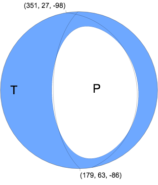
W-phase Moment Tensor (Mww)
Moment 2.992e+16 N-m
Magnitude 4.92 Mww
Depth 50.5 km
Percent DC 80%
Half Duration 0.74 s
Catalog US
Data Source US 3
Contributor US 3

Nodal Planes
Plane Strike Dip Rake
NP1 351 27 -98
NP2 179 63 -86

Principal Axes
Axis Value Plunge Azimuth
T 2.824e+16 N-m 18 266
N 0.312e+16 N-m 4 357
P -3.136e+16 N-m 72 98
|
Magnitudes
Given the availability of digital waveforms for determination of the moment tensor, this section documents the added processing leading to mLg, if appropriate to the region, and ML by application of the respective IASPEI formulae. As a research study, the linear distance term of the IASPEI formula
for ML is adjusted to remove a linear distance trend in residuals to give a regionally defined ML. The defined ML uses horizontal component recordings, but the same procedure is applied to the vertical components since there may be some interest in vertical component ground motions. Residual plots versus distance may indicate interesting features of ground motion scaling in some distance ranges. A residual plot of the regionalized magnitude is given as a function of distance and azimuth, since data sets may transcend different wave propagation provinces.
ML Magnitude
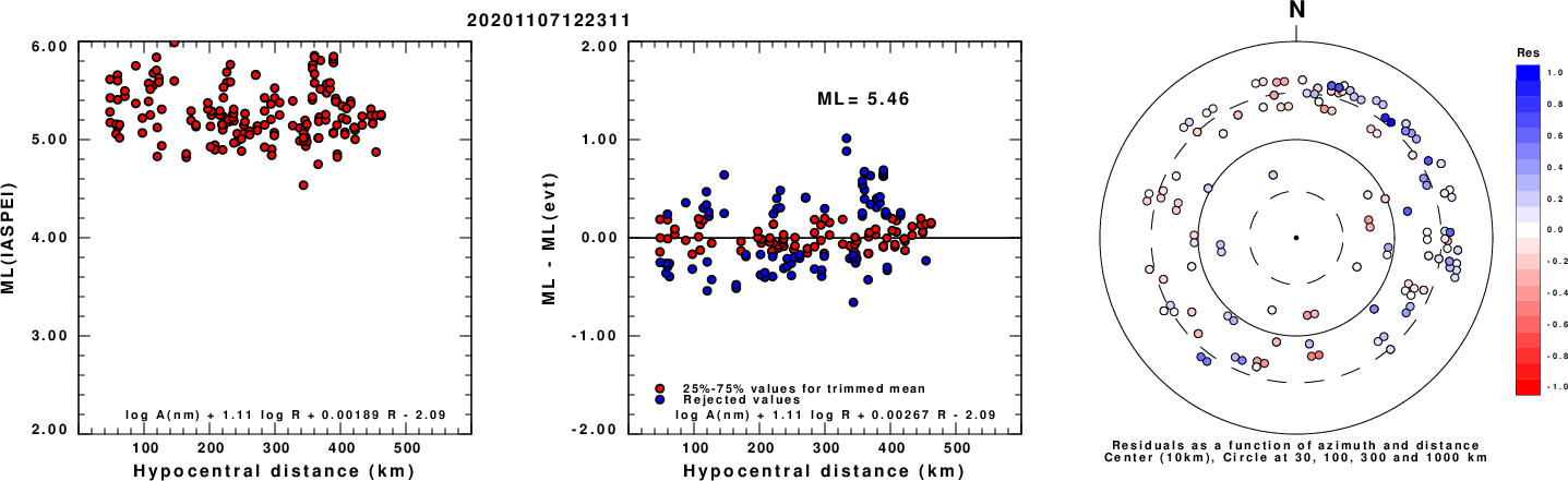
Left: ML computed using the IASPEI formula for Horizontal components. Center: ML residuals computed using a modified IASPEI formula that accounts for path specific attenuation; the values used for the trimmed mean are indicated. The ML relation used for each figure is given at the bottom of each plot.
Right: Residuals from new relation as a function of distance and azimuth.
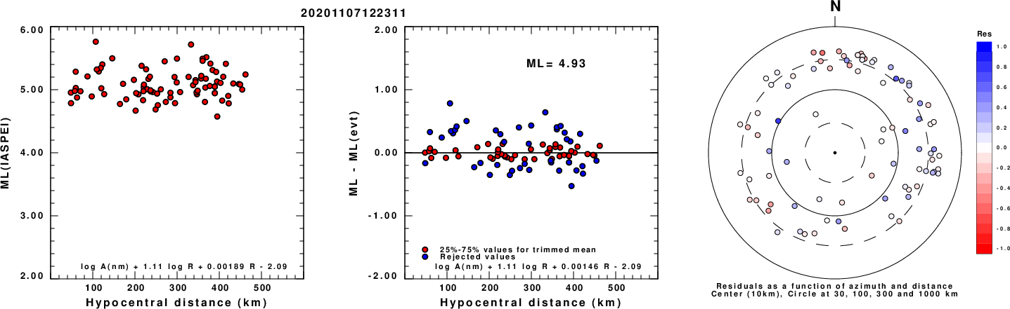
Left: ML computed using the IASPEI formula for Vertical components (research). Center: ML residuals computed using a modified IASPEI formula that accounts for path specific attenuation; the values used for the trimmed mean are indicated. The ML relation used for each figure is given at the bottom of each plot.
Right: Residuals from new relation as a function of distance and azimuth.
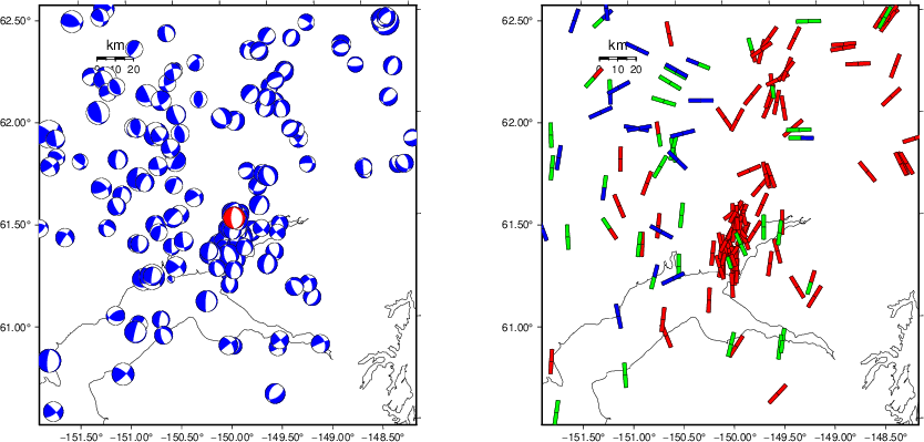
Context
The left panel of the next figure presents the focal mechanism for this earthquake (red) in the context of other nearby events (blue) in the SLU Moment Tensor Catalog. The right panel shows the inferred direction of maximum compressive stress and the type of faulting (green is strike-slip, red is normal, blue is thrust; oblique is shown by a combination of colors). Thus context plot is useful for assessing the appropriateness of the moment tensor of this event.
Waveform Inversion using wvfgrd96
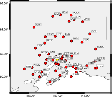
The focal mechanism was determined using broadband seismic waveforms. The location of the event (star) and the
stations used for (red) the waveform inversion are shown in the next figure.
|
|
Location of broadband stations used for waveform inversion
|
The program wvfgrd96 was used with good traces observed at short distance to determine the focal mechanism, depth and seismic moment. This technique requires a high quality signal and well determined velocity model for the Green's functions. To the extent that these are the quality data, this type of mechanism should be preferred over the radiation pattern technique which requires the separate step of defining the pressure and tension quadrants and the correct strike.
The observed and predicted traces are filtered using the following gsac commands:
cut o DIST/3.3 -40 o DIST/3.3 +50
rtr
taper w 0.1
hp c 0.03 n 3
lp c 0.10 n 3
The results of this grid search are as follow:
           DEPTH  STK   DIP  RAKE   MW    FIT
WVFGRD96    1.0     0    45    90   3.98 0.1542
WVFGRD96    2.0     0    45    90   4.14 0.2095
WVFGRD96    3.0   180    50    90   4.20 0.1920
WVFGRD96    4.0   155    75    65   4.18 0.1859
WVFGRD96    5.0   130    80   -50   4.20 0.2110
WVFGRD96    6.0   130    80   -50   4.22 0.2343
WVFGRD96    7.0   130    80   -45   4.25 0.2534
WVFGRD96    8.0   130    80   -55   4.32 0.2637
WVFGRD96    9.0   130    80   -50   4.34 0.2777
WVFGRD96   10.0   125    75   -50   4.36 0.2886
WVFGRD96   11.0   125    75   -50   4.38 0.2969
WVFGRD96   12.0   125    75   -50   4.39 0.3031
WVFGRD96   13.0   320    80    55   4.39 0.3094
WVFGRD96   14.0   120    25    70   4.41 0.3182
WVFGRD96   15.0   115    30    65   4.43 0.3272
WVFGRD96   16.0   115    30    65   4.45 0.3352
WVFGRD96   17.0   105    30    55   4.46 0.3418
WVFGRD96   18.0   100    30    45   4.47 0.3487
WVFGRD96   19.0   100    30    45   4.48 0.3550
WVFGRD96   20.0   100    30    45   4.50 0.3598
WVFGRD96   21.0   105    25    50   4.52 0.3664
WVFGRD96   22.0   105    25    50   4.53 0.3714
WVFGRD96   23.0   105    25    45   4.54 0.3753
WVFGRD96   24.0   110    20    50   4.55 0.3788
WVFGRD96   25.0   110    20    50   4.56 0.3810
WVFGRD96   26.0   110    20    50   4.57 0.3813
WVFGRD96   27.0   105    20    45   4.58 0.3804
WVFGRD96   28.0   105    20    45   4.59 0.3773
WVFGRD96   29.0    80    25    -5   4.59 0.3770
WVFGRD96   30.0    80    25   -10   4.60 0.3817
WVFGRD96   31.0    70    25   -20   4.61 0.3878
WVFGRD96   32.0    65    25   -25   4.62 0.3967
WVFGRD96   33.0    55    20   -35   4.63 0.4083
WVFGRD96   34.0    35    20   -55   4.64 0.4233
WVFGRD96   35.0    30    20   -60   4.65 0.4397
WVFGRD96   36.0    25    20   -65   4.66 0.4549
WVFGRD96   37.0    30    25   -60   4.66 0.4687
WVFGRD96   38.0    25    25   -65   4.67 0.4806
WVFGRD96   39.0    10    25   -80   4.68 0.4955
WVFGRD96   40.0   180    70   -90   4.81 0.5007
WVFGRD96   41.0     5    20   -85   4.82 0.5117
WVFGRD96   42.0     0    20   -90   4.83 0.5197
WVFGRD96   43.0    -5    25   -95   4.83 0.5277
WVFGRD96   44.0     0    25   -90   4.84 0.5349
WVFGRD96   45.0   180    65   -90   4.85 0.5417
WVFGRD96   46.0    -5    25   -95   4.86 0.5464
WVFGRD96   47.0   180    65   -90   4.86 0.5511
WVFGRD96   48.0    -5    25   -95   4.87 0.5543
WVFGRD96   49.0   180    65   -85   4.88 0.5558
WVFGRD96   50.0   -10    25  -100   4.88 0.5576
WVFGRD96   51.0   -10    25  -100   4.89 0.5578
WVFGRD96   52.0   180    65   -85   4.89 0.5552
WVFGRD96   53.0   180    65   -85   4.89 0.5538
WVFGRD96   54.0   -10    25  -100   4.89 0.5513
WVFGRD96   55.0   -10    25  -100   4.90 0.5474
WVFGRD96   56.0   180    65   -85   4.90 0.5426
WVFGRD96   57.0   180    65   -85   4.90 0.5375
WVFGRD96   58.0   180    65   -85   4.90 0.5322
WVFGRD96   59.0   180    65   -85   4.90 0.5265
The best solution is
WVFGRD96 51.0 -10 25 -100 4.89 0.5578
The mechanism corresponding to the best fit is
|
|
Figure 1. Waveform inversion focal mechanism
|
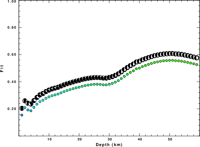
The best fit as a function of depth is given in the following figure:
|
|
Figure 2. Depth sensitivity for waveform mechanism
|
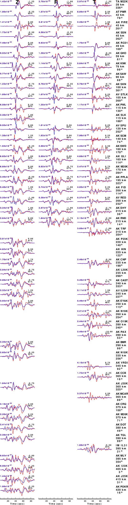
The comparison of the observed and predicted waveforms is given in the next figure. The red traces are the observed and the blue are the predicted.
Each observed-predicted component is plotted to the same scale and peak amplitudes are indicated by the numbers to the left of each trace. A pair of numbers is given in black at the right of each predicted traces. The upper number it the time shift required for maximum correlation between the observed and predicted traces. This time shift is required because the synthetics are not computed at exactly the same distance as the observed, the velocity model used in the predictions may not be perfect and the epicentral parameters may be be off.
A positive time shift indicates that the prediction is too fast and should be delayed to match the observed trace (shift to the right in this figure). A negative value indicates that the prediction is too slow. The lower number gives the percentage of variance reduction to characterize the individual goodness of fit (100% indicates a perfect fit).
The bandpass filter used in the processing and for the display was
cut o DIST/3.3 -40 o DIST/3.3 +50
rtr
taper w 0.1
hp c 0.03 n 3
lp c 0.10 n 3
|
|
Figure 3. Waveform comparison for selected depth. Red: observed; Blue - predicted. The time shift with respect to the model prediction is indicated. The percent of fit is also indicated. The time scale is relative to the first trace sample.
|
|
|
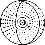
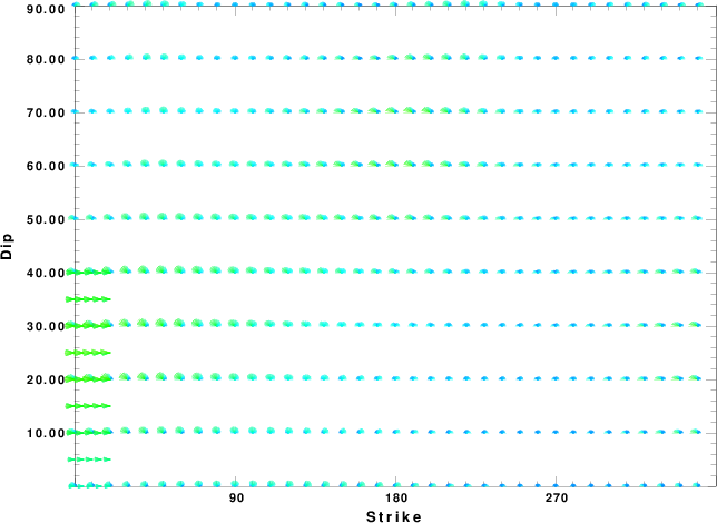
Focal mechanism sensitivity at the preferred depth. The red color indicates a very good fit to the waveforms.
Each solution is plotted as a vector at a given value of strike and dip with the angle of the vector representing the rake angle, measured, with respect to the upward vertical (N) in the figure.
|
A check on the assumed source location is possible by looking at the time shifts between the observed and predicted traces. The time shifts for waveform matching arise for several reasons:
- The origin time and epicentral distance are incorrect
- The velocity model used for the inversion is incorrect
- The velocity model used to define the P-arrival time is not the
same as the velocity model used for the waveform inversion
(assuming that the initial trace alignment is based on the
P arrival time)
Assuming only a mislocation, the time shifts are fit to a functional form:
Time_shift = A + B cos Azimuth + C Sin Azimuth
The time shifts for this inversion lead to the next figure:
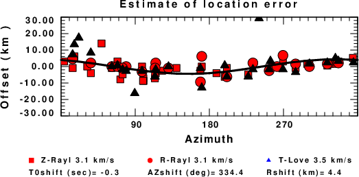
The derived shift in origin time and epicentral coordinates are given at the bottom of the figure.
Velocity Model
The WUS.model used for the waveform synthetic seismograms and for the surface wave eigenfunctions and dispersion is as follows
(The format is in the model96 format of Computer Programs in Seismology).
MODEL.01
Model after     8 iterations
ISOTROPIC
KGS
FLAT EARTH
1-D
CONSTANT VELOCITY
LINE08
LINE09
LINE10
LINE11
      H(KM)   VP(KM/S)   VS(KM/S) RHO(GM/CC)         QP         QS       ETAP       ETAS      FREFP      FREFS
     1.9000     3.4065     2.0089     2.2150  0.302E-02  0.679E-02   0.00       0.00       1.00       1.00
     6.1000     5.5445     3.2953     2.6089  0.349E-02  0.784E-02   0.00       0.00       1.00       1.00
    13.0000     6.2708     3.7396     2.7812  0.212E-02  0.476E-02   0.00       0.00       1.00       1.00
    19.0000     6.4075     3.7680     2.8223  0.111E-02  0.249E-02   0.00       0.00       1.00       1.00
     0.0000     7.9000     4.6200     3.2760  0.164E-10  0.370E-10   0.00       0.00       1.00       1.00
Last Changed Thu Apr 25 10:56:21 PM CDT 2024