Location
SLU Location
To check the ANSS location or to compare the observed P-wave first motions to the moment tensor solution, P- and S-wave first arrival times were manually read together with the P-wave first motions. The subsequent output of the program elocate is given in the file elocate.txt. The first motion plot is shown below.
Location ANSS
The ANSS event ID is us6000ccnk and the event page is at
https://earthquake.usgs.gov/earthquakes/eventpage/us6000ccnk/executive.
2020/10/24 16:18:47 62.252 -124.432 5.9 4.5 Canada, NWT
Focal Mechanism
 USGS/SLU Moment Tensor Solution
 ENS  2020/10/24 16:18:47:0  62.25 -124.43   5.9 4.5 Canada, NWT

 Stations used:
   1E.MONT2 1E.MONT7 1E.MONT9 AK.BESE AK.JIS AK.LOGN AK.PIN
   AK.PNL AK.R32K AK.S31K AK.S32K AK.U33K AK.V35K AT.SIT
   CN.BRWY CN.DAWY CN.DLBC CN.FNSB CN.FSJB CN.HYT CN.INK
   CN.KUKN CN.NAB1 CN.NAB2 CN.NAHA CN.NBC1 CN.NBC5 CN.NBC7
   CN.NBC8 CN.PLBC CN.WHY CN.YUK2 CN.YUK3 CN.YUK4 CN.YUK5
   CN.YUK6 CN.YUK7 CN.YUK8 EO.FSJ2 NY.MMPY NY.WGLY NY.WTLY
   RV.DEDWA TA.EPYK TA.F30M TA.F31M TA.G29M TA.G30M TA.H29M
   TA.H31M TA.I28M TA.I30M TA.J29N TA.J30M TA.K29M TA.L27K
   TA.L29M TA.M29M TA.M30M TA.M31M TA.N30M TA.N31M TA.O28M
   TA.O29M TA.O30N TA.P29M TA.P30M TA.P32M TA.P33M TA.Q32M
   TA.R31K TA.R33M TA.S34M TA.T33K TA.T35M US.WRAK

 Filtering commands used:
   cut o DIST/3.3 -40 o DIST/3.3 +50
   rtr
   taper w 0.1
   hp c 0.025 n 3
   lp c 0.06 n 3

 Best Fitting Double Couple
  Mo = 6.61e+22 dyne-cm
  Mw = 4.48
  Z  = 4 km
  Plane   Strike  Dip  Rake
   NP1      325    65    80
   NP2      168    27   110
  Principal Axes:
   Axis    Value   Plunge  Azimuth
    T   6.61e+22     68     215
    N   0.00e+00      9     329
    P  -6.61e+22     19      62

 Moment Tensor: (dyne-cm)
    Component   Value
       Mxx    -6.63e+21
       Mxy    -1.99e+22
       Mxz    -2.80e+22
       Myy    -4.32e+22
       Myz    -3.15e+22
       Mzz     4.98e+22


                     #-------------
                 ###-------------------
              ----##----------------------
             ---#######--------------------
           ----###########-------------------
          ----##############-------------   --
         ----################------------ P ---
        -----##################----------   ----
        -----####################---------------
       -----######################---------------
       -----#######################--------------
       ------#######################-------------
       ------##########   ###########------------
        -----########## T ############----------
        ------#########   ############----------
         ------########################--------
          ------########################------
           ------#######################-----
             ------#####################---
              -------###################--
                 ------################
                     ------########


 Global CMT Convention Moment Tensor:
      R          T          P
  4.98e+22  -2.80e+22   3.15e+22
 -2.80e+22  -6.63e+21   1.99e+22
  3.15e+22   1.99e+22  -4.32e+22


Details of the solution is found at

http://www.eas.slu.edu/eqc/eqc_mt/MECH.NA/20201024161847/index.html
|
Preferred Solution
The preferred solution from an analysis of the surface-wave spectral amplitude radiation pattern, waveform inversion or first motion observations is
      STK = 325
      DIP = 65
     RAKE = 80
       MW = 4.48
       HS = 4.0
The NDK file is 20201024161847.ndk
The waveform inversion is preferred.
Moment Tensor Comparison
The following compares this source inversion to those provided by others. The purpose is to look for major differences and also to note slight differences that might be inherent to the processing procedure. For completeness the USGS/SLU solution is repeated from above.
| SLU |
SLUFM |
 USGS/SLU Moment Tensor Solution
 ENS  2020/10/24 16:18:47:0  62.25 -124.43   5.9 4.5 Canada, NWT

 Stations used:
   1E.MONT2 1E.MONT7 1E.MONT9 AK.BESE AK.JIS AK.LOGN AK.PIN
   AK.PNL AK.R32K AK.S31K AK.S32K AK.U33K AK.V35K AT.SIT
   CN.BRWY CN.DAWY CN.DLBC CN.FNSB CN.FSJB CN.HYT CN.INK
   CN.KUKN CN.NAB1 CN.NAB2 CN.NAHA CN.NBC1 CN.NBC5 CN.NBC7
   CN.NBC8 CN.PLBC CN.WHY CN.YUK2 CN.YUK3 CN.YUK4 CN.YUK5
   CN.YUK6 CN.YUK7 CN.YUK8 EO.FSJ2 NY.MMPY NY.WGLY NY.WTLY
   RV.DEDWA TA.EPYK TA.F30M TA.F31M TA.G29M TA.G30M TA.H29M
   TA.H31M TA.I28M TA.I30M TA.J29N TA.J30M TA.K29M TA.L27K
   TA.L29M TA.M29M TA.M30M TA.M31M TA.N30M TA.N31M TA.O28M
   TA.O29M TA.O30N TA.P29M TA.P30M TA.P32M TA.P33M TA.Q32M
   TA.R31K TA.R33M TA.S34M TA.T33K TA.T35M US.WRAK

 Filtering commands used:
   cut o DIST/3.3 -40 o DIST/3.3 +50
   rtr
   taper w 0.1
   hp c 0.025 n 3
   lp c 0.06 n 3

 Best Fitting Double Couple
  Mo = 6.61e+22 dyne-cm
  Mw = 4.48
  Z  = 4 km
  Plane   Strike  Dip  Rake
   NP1      325    65    80
   NP2      168    27   110
  Principal Axes:
   Axis    Value   Plunge  Azimuth
    T   6.61e+22     68     215
    N   0.00e+00      9     329
    P  -6.61e+22     19      62

 Moment Tensor: (dyne-cm)
    Component   Value
       Mxx    -6.63e+21
       Mxy    -1.99e+22
       Mxz    -2.80e+22
       Myy    -4.32e+22
       Myz    -3.15e+22
       Mzz     4.98e+22


                     #-------------
                 ###-------------------
              ----##----------------------
             ---#######--------------------
           ----###########-------------------
          ----##############-------------   --
         ----################------------ P ---
        -----##################----------   ----
        -----####################---------------
       -----######################---------------
       -----#######################--------------
       ------#######################-------------
       ------##########   ###########------------
        -----########## T ############----------
        ------#########   ############----------
         ------########################--------
          ------########################------
           ------#######################-----
             ------#####################---
              -------###################--
                 ------################
                     ------########


 Global CMT Convention Moment Tensor:
      R          T          P
  4.98e+22  -2.80e+22   3.15e+22
 -2.80e+22  -6.63e+21   1.99e+22
  3.15e+22   1.99e+22  -4.32e+22


Details of the solution is found at

http://www.eas.slu.edu/eqc/eqc_mt/MECH.NA/20201024161847/index.html
|
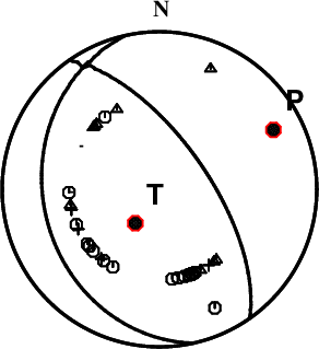
First motions and takeoff angles from an elocate run.
|
Magnitudes
Given the availability of digital waveforms for determination of the moment tensor, this section documents the added processing leading to mLg, if appropriate to the region, and ML by application of the respective IASPEI formulae. As a research study, the linear distance term of the IASPEI formula
for ML is adjusted to remove a linear distance trend in residuals to give a regionally defined ML. The defined ML uses horizontal component recordings, but the same procedure is applied to the vertical components since there may be some interest in vertical component ground motions. Residual plots versus distance may indicate interesting features of ground motion scaling in some distance ranges. A residual plot of the regionalized magnitude is given as a function of distance and azimuth, since data sets may transcend different wave propagation provinces.
mLg Magnitude
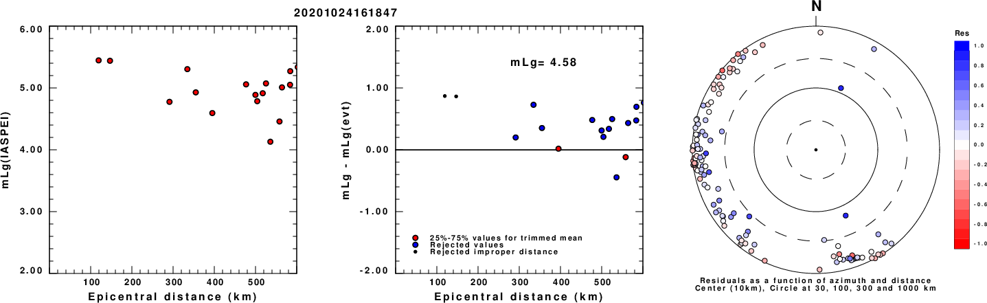
Left: mLg computed using the IASPEI formula. Center: mLg residuals versus epicentral distance ; the values used for the trimmed mean magnitude estimate are indicated.
Right: residuals as a function of distance and azimuth.
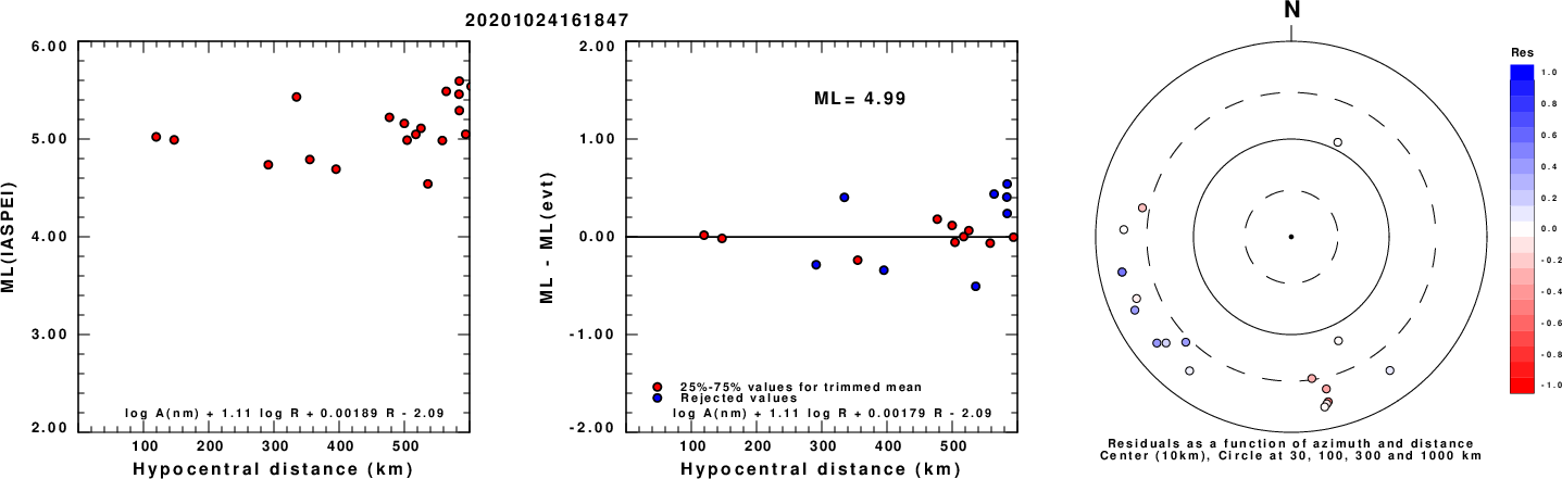
ML Magnitude
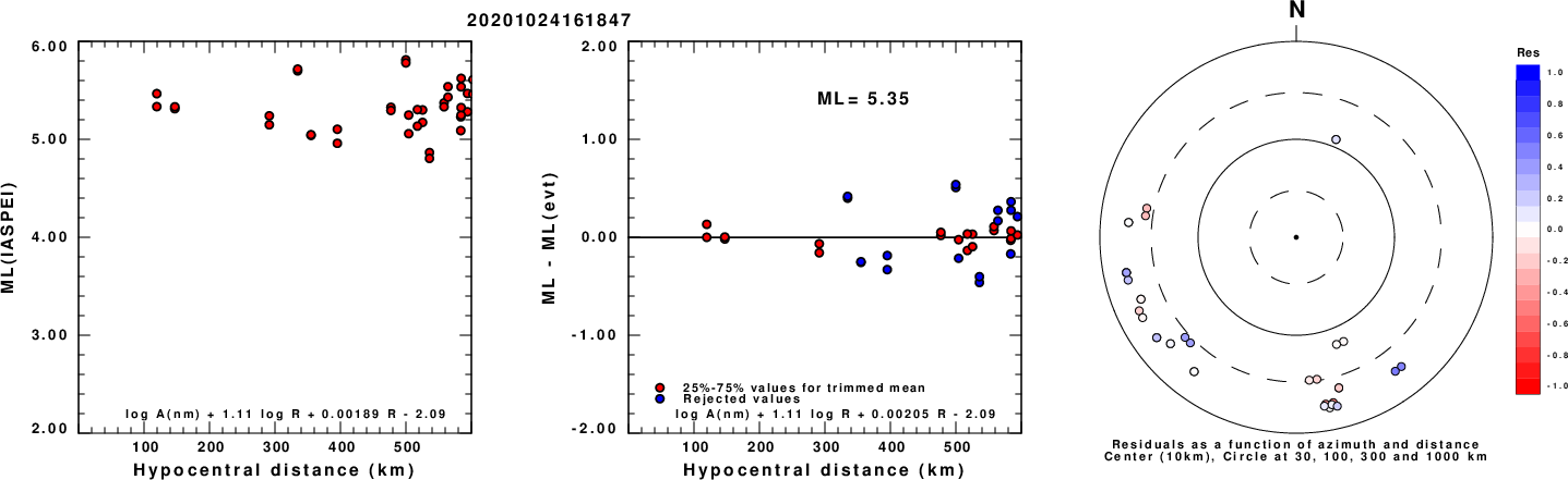
Left: ML computed using the IASPEI formula for Horizontal components. Center: ML residuals computed using a modified IASPEI formula that accounts for path specific attenuation; the values used for the trimmed mean are indicated. The ML relation used for each figure is given at the bottom of each plot.
Right: Residuals from new relation as a function of distance and azimuth.
Left: ML computed using the IASPEI formula for Vertical components (research). Center: ML residuals computed using a modified IASPEI formula that accounts for path specific attenuation; the values used for the trimmed mean are indicated. The ML relation used for each figure is given at the bottom of each plot.
Right: Residuals from new relation as a function of distance and azimuth.
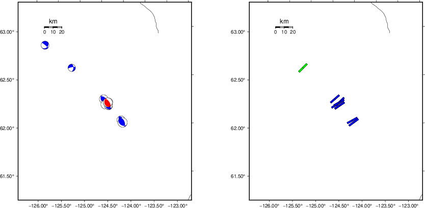
Context
The left panel of the next figure presents the focal mechanism for this earthquake (red) in the context of other nearby events (blue) in the SLU Moment Tensor Catalog. The right panel shows the inferred direction of maximum compressive stress and the type of faulting (green is strike-slip, red is normal, blue is thrust; oblique is shown by a combination of colors). Thus context plot is useful for assessing the appropriateness of the moment tensor of this event.
Waveform Inversion using wvfgrd96
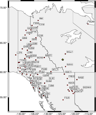
The focal mechanism was determined using broadband seismic waveforms. The location of the event (star) and the
stations used for (red) the waveform inversion are shown in the next figure.
|
|
Location of broadband stations used for waveform inversion
|
The program wvfgrd96 was used with good traces observed at short distance to determine the focal mechanism, depth and seismic moment. This technique requires a high quality signal and well determined velocity model for the Green's functions. To the extent that these are the quality data, this type of mechanism should be preferred over the radiation pattern technique which requires the separate step of defining the pressure and tension quadrants and the correct strike.
The observed and predicted traces are filtered using the following gsac commands:
cut o DIST/3.3 -40 o DIST/3.3 +50
rtr
taper w 0.1
hp c 0.025 n 3
lp c 0.06 n 3
The results of this grid search are as follow:
           DEPTH  STK   DIP  RAKE   MW    FIT
WVFGRD96    1.0   305    80    75   4.55 0.6777
WVFGRD96    2.0   310    75    75   4.50 0.6808
WVFGRD96    3.0   315    70    75   4.47 0.6868
WVFGRD96    4.0   325    65    80   4.48 0.6891
WVFGRD96    5.0   155    25    95   4.48 0.6835
WVFGRD96    6.0   155    30    95   4.48 0.6678
WVFGRD96    7.0   155    30    95   4.46 0.6479
WVFGRD96    8.0   330    60    90   4.45 0.6244
WVFGRD96    9.0   265    50   -55   4.44 0.6282
WVFGRD96   10.0   265    50   -55   4.46 0.6277
WVFGRD96   11.0   265    50   -55   4.46 0.6355
WVFGRD96   12.0   265    50   -55   4.46 0.6363
WVFGRD96   13.0   265    50   -55   4.45 0.6316
WVFGRD96   14.0   270    50   -50   4.45 0.6233
WVFGRD96   15.0   270    50   -50   4.45 0.6136
WVFGRD96   16.0   270    50   -50   4.45 0.6024
WVFGRD96   17.0   270    50   -50   4.45 0.5906
WVFGRD96   18.0   270    50   -50   4.45 0.5788
WVFGRD96   19.0   270    50   -50   4.45 0.5671
WVFGRD96   20.0   270    50   -50   4.47 0.5508
WVFGRD96   21.0   270    50   -50   4.47 0.5360
WVFGRD96   22.0   335    55   -80   4.46 0.5252
WVFGRD96   23.0   335    55   -80   4.46 0.5166
WVFGRD96   24.0   335    55   -80   4.46 0.5072
WVFGRD96   25.0   335    55   -80   4.47 0.4976
WVFGRD96   26.0   340    55   -75   4.47 0.4880
WVFGRD96   27.0   340    55   -75   4.47 0.4780
WVFGRD96   28.0   340    55   -75   4.47 0.4679
WVFGRD96   29.0   340    55   -75   4.48 0.4577
The best solution is
WVFGRD96 4.0 325 65 80 4.48 0.6891
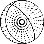
The mechanism corresponding to the best fit is
|
|
Figure 1. Waveform inversion focal mechanism
|
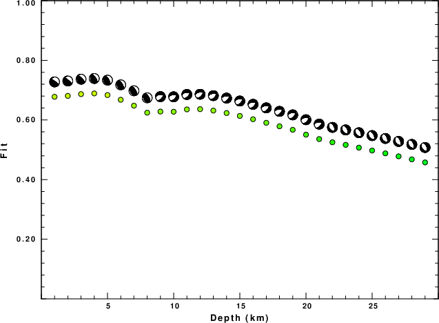
The best fit as a function of depth is given in the following figure:
|
|
Figure 2. Depth sensitivity for waveform mechanism
|
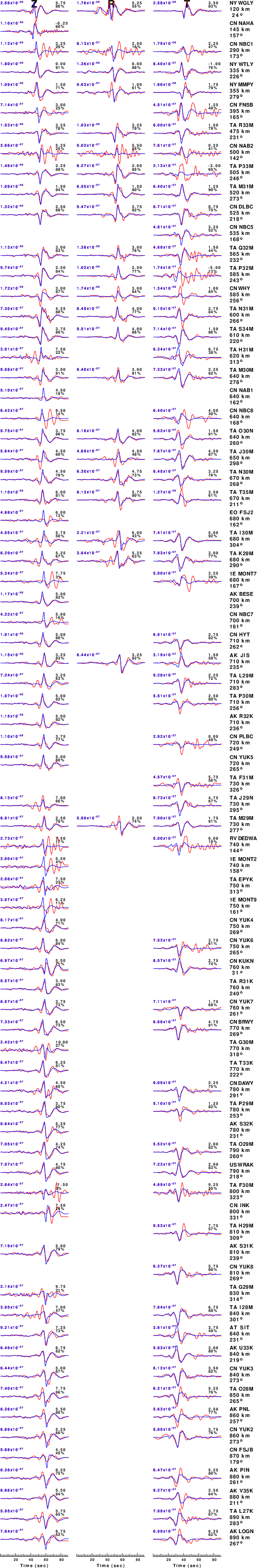
The comparison of the observed and predicted waveforms is given in the next figure. The red traces are the observed and the blue are the predicted.
Each observed-predicted component is plotted to the same scale and peak amplitudes are indicated by the numbers to the left of each trace. A pair of numbers is given in black at the right of each predicted traces. The upper number it the time shift required for maximum correlation between the observed and predicted traces. This time shift is required because the synthetics are not computed at exactly the same distance as the observed, the velocity model used in the predictions may not be perfect and the epicentral parameters may be be off.
A positive time shift indicates that the prediction is too fast and should be delayed to match the observed trace (shift to the right in this figure). A negative value indicates that the prediction is too slow. The lower number gives the percentage of variance reduction to characterize the individual goodness of fit (100% indicates a perfect fit).
The bandpass filter used in the processing and for the display was
cut o DIST/3.3 -40 o DIST/3.3 +50
rtr
taper w 0.1
hp c 0.025 n 3
lp c 0.06 n 3
|
|
Figure 3. Waveform comparison for selected depth. Red: observed; Blue - predicted. The time shift with respect to the model prediction is indicated. The percent of fit is also indicated. The time scale is relative to the first trace sample.
|
|
|
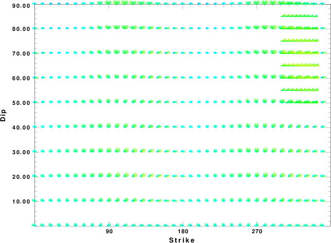
Focal mechanism sensitivity at the preferred depth. The red color indicates a very good fit to the waveforms.
Each solution is plotted as a vector at a given value of strike and dip with the angle of the vector representing the rake angle, measured, with respect to the upward vertical (N) in the figure.
|
A check on the assumed source location is possible by looking at the time shifts between the observed and predicted traces. The time shifts for waveform matching arise for several reasons:
- The origin time and epicentral distance are incorrect
- The velocity model used for the inversion is incorrect
- The velocity model used to define the P-arrival time is not the
same as the velocity model used for the waveform inversion
(assuming that the initial trace alignment is based on the
P arrival time)
Assuming only a mislocation, the time shifts are fit to a functional form:
Time_shift = A + B cos Azimuth + C Sin Azimuth
The time shifts for this inversion lead to the next figure:
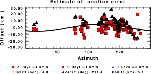
The derived shift in origin time and epicentral coordinates are given at the bottom of the figure.
Velocity Model
The CUS.model used for the waveform synthetic seismograms and for the surface wave eigenfunctions and dispersion is as follows
(The format is in the model96 format of Computer Programs in Seismology).
MODEL.01
CUS Model with Q from simple gamma values
ISOTROPIC
KGS
FLAT EARTH
1-D
CONSTANT VELOCITY
LINE08
LINE09
LINE10
LINE11
  H(KM) VP(KM/S) VS(KM/S) RHO(GM/CC)   QP   QS  ETAP  ETAS  FREFP  FREFS
  1.0000  5.0000  2.8900  2.5000 0.172E-02 0.387E-02 0.00  0.00  1.00  1.00
  9.0000  6.1000  3.5200  2.7300 0.160E-02 0.363E-02 0.00  0.00  1.00  1.00
 10.0000  6.4000  3.7000  2.8200 0.149E-02 0.336E-02 0.00  0.00  1.00  1.00
 20.0000  6.7000  3.8700  2.9020 0.000E-04 0.000E-04 0.00  0.00  1.00  1.00
  0.0000  8.1500  4.7000  3.3640 0.194E-02 0.431E-02 0.00  0.00  1.00  1.00
Last Changed Thu Apr 25 10:35:34 PM CDT 2024