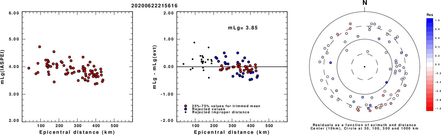
Left: mLg computed using the IASPEI formula. Center: mLg residuals versus epicentral distance ; the values used for the trimmed mean magnitude estimate are indicated. Right: residuals as a function of distance and azimuth.
The ANSS event ID is ak020804cj04 and the event page is at https://earthquake.usgs.gov/earthquakes/eventpage/ak020804cj04/executive.
2020/06/22 21:56:16 64.689 -150.889 24.1 3.8 Alaska
 USGS/SLU Moment Tensor Solution
 ENS  2020/06/22 21:56:16:0  64.69 -150.89  24.1 3.8 Alaska

 Stations used:
   AK.CAST AK.CCB AK.DHY AK.H21K AK.H22K AK.H23K AK.H24K
   AK.HDA AK.I21K AK.I23K AK.I26K AK.J17K AK.J19K AK.J20K
   AK.J25K AK.K20K AK.KLU AK.KNK AK.L18K AK.L19K AK.L22K
   AK.L26K AK.M20K AK.MCK AK.MLY AK.NEA2 AK.PAX AK.PPD AK.PPLA
   AK.RIDG AK.RND AK.TRF AK.WRH AT.MENT AT.PMR AV.STLK IM.IL31
   IU.COLA TA.E21K TA.E23K TA.E24K TA.F19K TA.F20K TA.F21K
   TA.F24K TA.F25K TA.G18K TA.G19K TA.G21K TA.G23K TA.G24K
   TA.G26K TA.H17K TA.H18K TA.H19K TA.I20K TA.K17K

 Filtering commands used:
   cut o DIST/3.3 -40 o DIST/3.3 +50
   rtr
   taper w 0.1
   hp c 0.03 n 3
   lp c 0.10 n 3

 Best Fitting Double Couple
  Mo = 4.32e+21 dyne-cm
  Mw = 3.69
  Z  = 22 km
  Plane   Strike  Dip  Rake
   NP1      180    70   -50
   NP2      292    44   -150
  Principal Axes:
   Axis    Value   Plunge  Azimuth
    T   4.32e+21     15     242
    N   0.00e+00     37     344
    P  -4.32e+21     49     133

 Moment Tensor: (dyne-cm)
    Component   Value
       Mxx    -4.56e+14
       Mxy     2.61e+21
       Mxz     9.49e+20
       Myy     2.12e+21
       Myz    -2.53e+21
       Mzz    -2.12e+21


                     ------########
                 ---------#############
              -----------#################
             ------------##################
           ------#######----#################
          --############---------#############
         ###############-------------##########
        ###############----------------#########
        ###############------------------#######
       ################--------------------######
       ################---------------------#####
       ################----------------------####
       ################-----------------------###
        ###############-----------   ----------#
        ###   #########----------- P ----------#
         ## T ##########----------   ----------
          #   ##########----------------------
           #############---------------------
             ############------------------
              ###########-----------------
                 #########-------------
                     ######--------


 Global CMT Convention Moment Tensor:
      R          T          P
 -2.12e+21   9.49e+20   2.53e+21
  9.49e+20  -4.56e+14  -2.61e+21
  2.53e+21  -2.61e+21   2.12e+21


Details of the solution is found at

http://www.eas.slu.edu/eqc/eqc_mt/MECH.NA/20200622215616/index.html
|
      STK = 180
      DIP = 70
     RAKE = -50
       MW = 3.69
       HS = 22.0
The NDK file is 20200622215616.ndk The waveform inversion is preferred.
Given the availability of digital waveforms for determination of the moment tensor, this section documents the added processing leading to mLg, if appropriate to the region, and ML by application of the respective IASPEI formulae. As a research study, the linear distance term of the IASPEI formula for ML is adjusted to remove a linear distance trend in residuals to give a regionally defined ML. The defined ML uses horizontal component recordings, but the same procedure is applied to the vertical components since there may be some interest in vertical component ground motions. Residual plots versus distance may indicate interesting features of ground motion scaling in some distance ranges. A residual plot of the regionalized magnitude is given as a function of distance and azimuth, since data sets may transcend different wave propagation provinces.
Left: mLg computed using the IASPEI formula. Center: mLg residuals versus epicentral distance ; the values used for the trimmed mean magnitude estimate are indicated.
Right: residuals as a function of distance and azimuth.
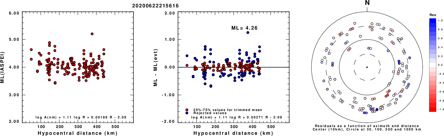
Left: ML computed using the IASPEI formula for Horizontal components. Center: ML residuals computed using a modified IASPEI formula that accounts for path specific attenuation; the values used for the trimmed mean are indicated. The ML relation used for each figure is given at the bottom of each plot.
Right: Residuals from new relation as a function of distance and azimuth.
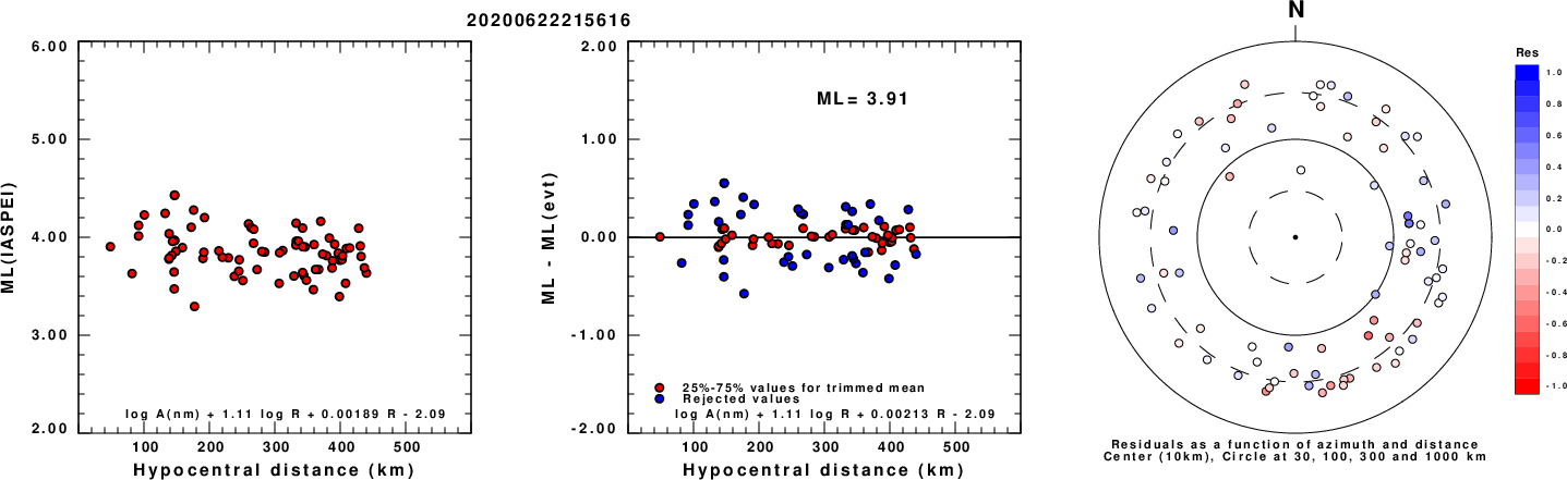
Left: ML computed using the IASPEI formula for Vertical components (research). Center: ML residuals computed using a modified IASPEI formula that accounts for path specific attenuation; the values used for the trimmed mean are indicated. The ML relation used for each figure is given at the bottom of each plot.
Right: Residuals from new relation as a function of distance and azimuth.
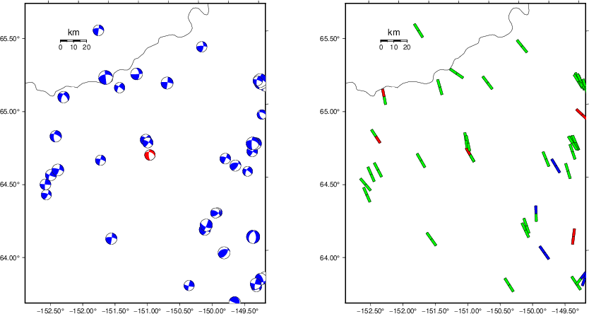 |
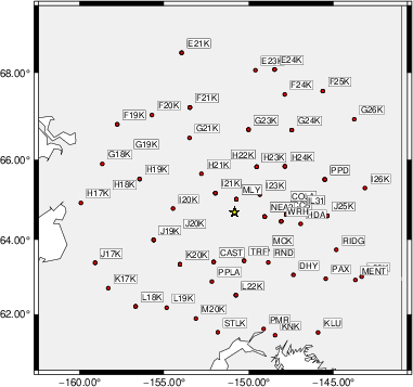
The focal mechanism was determined using broadband seismic waveforms. The location of the event (star) and the stations used for (red) the waveform inversion are shown in the next figure.
|
|
|
The program wvfgrd96 was used with good traces observed at short distance to determine the focal mechanism, depth and seismic moment. This technique requires a high quality signal and well determined velocity model for the Green's functions. To the extent that these are the quality data, this type of mechanism should be preferred over the radiation pattern technique which requires the separate step of defining the pressure and tension quadrants and the correct strike.
The observed and predicted traces are filtered using the following gsac commands:
cut o DIST/3.3 -40 o DIST/3.3 +50
rtr
taper w 0.1
hp c 0.03 n 3
lp c 0.10 n 3
The results of this grid search are as follow:
           DEPTH  STK   DIP  RAKE   MW    FIT
WVFGRD96    1.0   335    45    90   3.14 0.2349
WVFGRD96    2.0   155    45    90   3.30 0.3211
WVFGRD96    3.0   145    45    80   3.32 0.2595
WVFGRD96    4.0   285    60   -10   3.25 0.2494
WVFGRD96    5.0   280    55   -15   3.28 0.2616
WVFGRD96    6.0   280    50   -10   3.30 0.2770
WVFGRD96    7.0    15    80    45   3.33 0.3066
WVFGRD96    8.0    20    80    45   3.40 0.3349
WVFGRD96    9.0    20    75    45   3.43 0.3660
WVFGRD96   10.0    20    75    45   3.46 0.3954
WVFGRD96   11.0   185    75   -45   3.48 0.4278
WVFGRD96   12.0   185    70   -45   3.51 0.4636
WVFGRD96   13.0   185    70   -45   3.54 0.4984
WVFGRD96   14.0   180    65   -45   3.56 0.5317
WVFGRD96   15.0   180    65   -45   3.58 0.5624
WVFGRD96   16.0   180    65   -45   3.60 0.5894
WVFGRD96   17.0   180    65   -45   3.62 0.6123
WVFGRD96   18.0   180    70   -45   3.64 0.6315
WVFGRD96   19.0   180    70   -45   3.65 0.6473
WVFGRD96   20.0   180    70   -45   3.67 0.6581
WVFGRD96   21.0   180    70   -50   3.68 0.6647
WVFGRD96   22.0   180    70   -50   3.69 0.6681
WVFGRD96   23.0   180    70   -50   3.70 0.6662
WVFGRD96   24.0   180    70   -50   3.71 0.6618
WVFGRD96   25.0   180    70   -50   3.72 0.6539
WVFGRD96   26.0   175    70   -55   3.73 0.6443
WVFGRD96   27.0   180    75   -55   3.73 0.6328
WVFGRD96   28.0   180    75   -55   3.74 0.6200
WVFGRD96   29.0   180    75   -55   3.74 0.6056
WVFGRD96   30.0   180    75   -55   3.75 0.5909
WVFGRD96   31.0   180    75   -55   3.75 0.5727
WVFGRD96   32.0   180    75   -55   3.75 0.5561
WVFGRD96   33.0   185    80   -55   3.75 0.5387
WVFGRD96   34.0   185    80   -55   3.76 0.5222
WVFGRD96   35.0   185    80   -55   3.76 0.5079
WVFGRD96   36.0   185    80   -55   3.76 0.4928
WVFGRD96   37.0   185    80   -55   3.76 0.4798
WVFGRD96   38.0   185    80   -55   3.76 0.4679
WVFGRD96   39.0   180    80   -50   3.77 0.4569
WVFGRD96   40.0   180    80   -60   3.87 0.4432
WVFGRD96   41.0   180    80   -60   3.87 0.4309
WVFGRD96   42.0   185    80   -55   3.87 0.4187
WVFGRD96   43.0   185    80   -55   3.87 0.4074
WVFGRD96   44.0   185    80   -50   3.87 0.3979
WVFGRD96   45.0   185    80   -50   3.87 0.3883
WVFGRD96   46.0   175    80   -50   3.88 0.3794
WVFGRD96   47.0   175    80   -50   3.88 0.3717
WVFGRD96   48.0   175    80   -50   3.88 0.3635
WVFGRD96   49.0   175    80   -50   3.89 0.3567
WVFGRD96   50.0   175    80   -45   3.89 0.3485
WVFGRD96   51.0   175    80   -45   3.89 0.3420
WVFGRD96   52.0   175    80   -45   3.89 0.3348
WVFGRD96   53.0   175    80   -45   3.89 0.3285
WVFGRD96   54.0   175    80   -45   3.90 0.3234
WVFGRD96   55.0   175    80   -45   3.90 0.3177
WVFGRD96   56.0   175    80   -45   3.90 0.3132
WVFGRD96   57.0   175    80   -45   3.90 0.3093
WVFGRD96   58.0   175    80   -45   3.90 0.3045
WVFGRD96   59.0   175    80   -45   3.91 0.3009
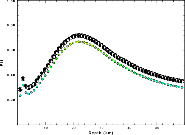
The best solution is
WVFGRD96 22.0 180 70 -50 3.69 0.6681
The mechanism corresponding to the best fit is
|
|
|
The best fit as a function of depth is given in the following figure:
|
|
|
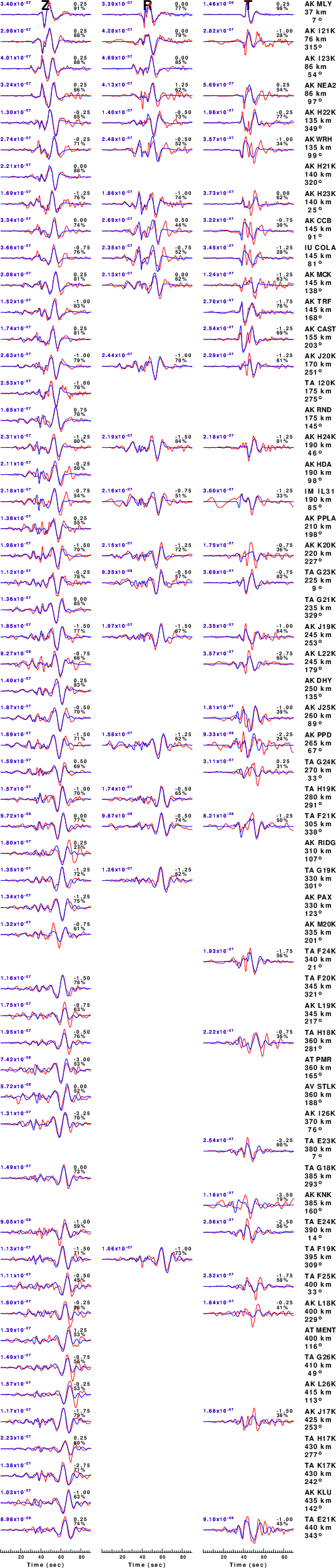
The comparison of the observed and predicted waveforms is given in the next figure. The red traces are the observed and the blue are the predicted. Each observed-predicted component is plotted to the same scale and peak amplitudes are indicated by the numbers to the left of each trace. A pair of numbers is given in black at the right of each predicted traces. The upper number it the time shift required for maximum correlation between the observed and predicted traces. This time shift is required because the synthetics are not computed at exactly the same distance as the observed, the velocity model used in the predictions may not be perfect and the epicentral parameters may be be off. A positive time shift indicates that the prediction is too fast and should be delayed to match the observed trace (shift to the right in this figure). A negative value indicates that the prediction is too slow. The lower number gives the percentage of variance reduction to characterize the individual goodness of fit (100% indicates a perfect fit).
The bandpass filter used in the processing and for the display was
cut o DIST/3.3 -40 o DIST/3.3 +50
rtr
taper w 0.1
hp c 0.03 n 3
lp c 0.10 n 3
|
| Figure 3. Waveform comparison for selected depth. Red: observed; Blue - predicted. The time shift with respect to the model prediction is indicated. The percent of fit is also indicated. The time scale is relative to the first trace sample. |
|
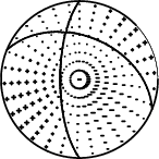
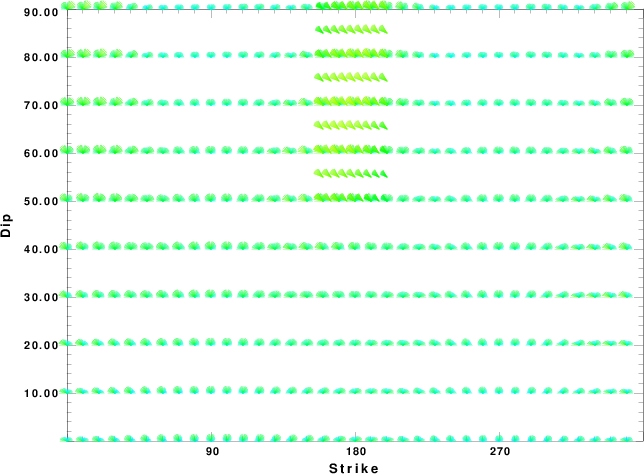
| Focal mechanism sensitivity at the preferred depth. The red color indicates a very good fit to the waveforms. Each solution is plotted as a vector at a given value of strike and dip with the angle of the vector representing the rake angle, measured, with respect to the upward vertical (N) in the figure. |
A check on the assumed source location is possible by looking at the time shifts between the observed and predicted traces. The time shifts for waveform matching arise for several reasons:
Time_shift = A + B cos Azimuth + C Sin Azimuth
The time shifts for this inversion lead to the next figure:
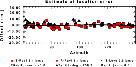
The derived shift in origin time and epicentral coordinates are given at the bottom of the figure.
The WUS.model used for the waveform synthetic seismograms and for the surface wave eigenfunctions and dispersion is as follows (The format is in the model96 format of Computer Programs in Seismology).
MODEL.01
Model after     8 iterations
ISOTROPIC
KGS
FLAT EARTH
1-D
CONSTANT VELOCITY
LINE08
LINE09
LINE10
LINE11
      H(KM)   VP(KM/S)   VS(KM/S) RHO(GM/CC)         QP         QS       ETAP       ETAS      FREFP      FREFS
     1.9000     3.4065     2.0089     2.2150  0.302E-02  0.679E-02   0.00       0.00       1.00       1.00
     6.1000     5.5445     3.2953     2.6089  0.349E-02  0.784E-02   0.00       0.00       1.00       1.00
    13.0000     6.2708     3.7396     2.7812  0.212E-02  0.476E-02   0.00       0.00       1.00       1.00
    19.0000     6.4075     3.7680     2.8223  0.111E-02  0.249E-02   0.00       0.00       1.00       1.00
     0.0000     7.9000     4.6200     3.2760  0.164E-10  0.370E-10   0.00       0.00       1.00       1.00