Location

Location ANSS

The ANSS event ID is uu60363602 and the event page is at https://earthquake.usgs.gov/earthquakes/eventpage/uu60363602/executive.

2020/03/18 13:09:31 40.751 -112.078 11.9 5.7 Utah

Focal Mechanism

USGS/SLU Moment Tensor Solution ENS 2020/03/18 13:09:31:0 40.75 -112.08 11.9 5.7 Utah Stations used: IW.FLWY IW.FXWY IW.LOHW IW.MFID IW.MOOW IW.SNOW N4.O20A NN.PIO US.AHID US.BW06 US.DUG US.ELK US.HLID US.HWUT UU.BGU UU.BRPU UU.BRWY UU.BSUT UU.CCUT UU.CTU UU.CVRU UU.ECUT UU.HMU UU.HVU UU.KNB UU.LCMT UU.LIUT UU.MPU UU.MTPU UU.NLU UU.PKCU UU.PNSU UU.PSUT UU.RDMU UU.SPU UU.SRU UU.SVWY UU.SZCU UU.TCRU UU.TCU UU.VRUT WY.YFT WY.YMR WY.YPP Filtering commands used: cut o DIST/3.3 -40 o DIST/3.3 +50 rtr taper w 0.1 hp c 0.03 n 3 lp c 0.10 n 3 Best Fitting Double Couple Mo = 2.02e+24 dyne-cm Mw = 5.47 Z = 12 km Plane Strike Dip Rake NP1 325 60 -109 NP2 180 35 -60 Principal Axes: Axis Value Plunge Azimuth T 2.02e+24 13 69 N 0.00e+00 17 335 P -2.02e+24 69 195 Moment Tensor: (dyne-cm) Component Value Mxx -1.01e+17 Mxy 5.79e+23 Mxz 8.27e+23 Myy 1.64e+24 Myz 5.98e+23 Mzz -1.64e+24 ----########## -----################# ######-##################### ######-----################### #######---------################## #######------------################# #######---------------############ # #######------------------########## T ## #######-------------------######### ## ########--------------------############## #######----------------------############# #######-----------------------############ ########---------- ----------########### #######---------- P -----------######### #######---------- -----------######### #######------------------------####### #######-----------------------###### #######----------------------##### ######---------------------### ######--------------------## #####----------------- ####---------- Global CMT Convention Moment Tensor: R T P -1.64e+24 8.27e+23 -5.98e+23 8.27e+23 -1.01e+17 -5.79e+23 -5.98e+23 -5.79e+23 1.64e+24 Details of the solution is found at http://www.eas.slu.edu/eqc/eqc_mt/MECH.NA/20200318130931/index.html

Preferred Solution

      STK = 180
      DIP = 35
     RAKE = -60
       MW = 5.47
       HS = 12.0

The NDK file is 20200318130931.ndk The waveform inversion is preferred.

Moment Tensor Comparison

The following compares this source inversion to those provided by others. The purpose is to look for major differences and also to note slight differences that might be inherent to the processing procedure. For completeness the USGS/SLU solution is repeated from above.

SLU	USGSMWR	USGSW	UUSS
USGS/SLU Moment Tensor Solution ENS 2020/03/18 13:09:31:0 40.75 -112.08 11.9 5.7 Utah Stations used: IW.FLWY IW.FXWY IW.LOHW IW.MFID IW.MOOW IW.SNOW N4.O20A NN.PIO US.AHID US.BW06 US.DUG US.ELK US.HLID US.HWUT UU.BGU UU.BRPU UU.BRWY UU.BSUT UU.CCUT UU.CTU UU.CVRU UU.ECUT UU.HMU UU.HVU UU.KNB UU.LCMT UU.LIUT UU.MPU UU.MTPU UU.NLU UU.PKCU UU.PNSU UU.PSUT UU.RDMU UU.SPU UU.SRU UU.SVWY UU.SZCU UU.TCRU UU.TCU UU.VRUT WY.YFT WY.YMR WY.YPP Filtering commands used: cut o DIST/3.3 -40 o DIST/3.3 +50 rtr taper w 0.1 hp c 0.03 n 3 lp c 0.10 n 3 Best Fitting Double Couple Mo = 2.02e+24 dyne-cm Mw = 5.47 Z = 12 km Plane Strike Dip Rake NP1 325 60 -109 NP2 180 35 -60 Principal Axes: Axis Value Plunge Azimuth T 2.02e+24 13 69 N 0.00e+00 17 335 P -2.02e+24 69 195 Moment Tensor: (dyne-cm) Component Value Mxx -1.01e+17 Mxy 5.79e+23 Mxz 8.27e+23 Myy 1.64e+24 Myz 5.98e+23 Mzz -1.64e+24 ----########## -----################# ######-##################### ######-----################### #######---------################## #######------------################# #######---------------############ # #######------------------########## T ## #######-------------------######### ## ########--------------------############## #######----------------------############# #######-----------------------############ ########---------- ----------########### #######---------- P -----------######### #######---------- -----------######### #######------------------------####### #######-----------------------###### #######----------------------##### ######---------------------### ######--------------------## #####----------------- ####---------- Global CMT Convention Moment Tensor: R T P -1.64e+24 8.27e+23 -5.98e+23 8.27e+23 -1.01e+17 -5.79e+23 -5.98e+23 -5.79e+23 1.64e+24 Details of the solution is found at http://www.eas.slu.edu/eqc/eqc_mt/MECH.NA/20200318130931/index.html	Regional Moment Tensor (Mwr) Moment 2.742e+17 N-m Magnitude 5.56 Mwr Depth 9.0 km Percent DC 89% Half Duration - Catalog US Data Source US 2 Contributor US 2 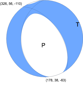Nodal Planes Plane Strike Dip Rake NP1 178 38 -63 NP2 326 56 -110 Principal Axes Axis Value Plunge Azimuth T 2.659e+17 N-m 9 70 N 0.159e+17 N-m 16 337 P -2.818e+17 N-m 71 189	W-phase Moment Tensor (Mww) Moment 3.949e+17 N-m Magnitude 5.66 Mww Depth 15.5 km Percent DC 93% Half Duration 1.67 s Catalog US Data Source US 1 Contributor US 1 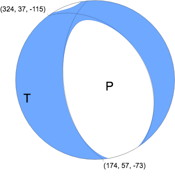Nodal Planes Plane Strike Dip Rake NP1 324 37 -115 NP2 174 57 -73 Principal Axes Axis Value Plunge Azimuth T 3.878e+17 N-m 11 252 N 0.138e+17 N-m 15 345 P -4.017e+17 N-m 72 127	Moment Tensor (TDMT) Moment 2.288e+17 N-m Magnitude 5.51 Depth 9.0 km Percent DC 95% Half Duration - Catalog UU Data Source UU 3 Contributor UU 3 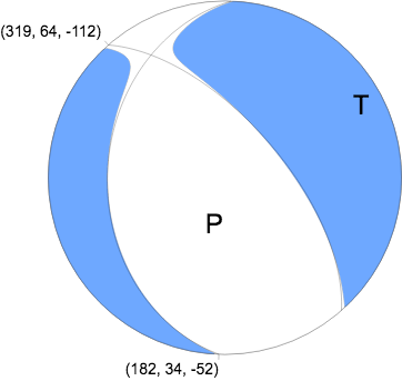Nodal Planes Plane Strike Dip Rake NP1 182 34 -52 NP2 319 64 -112 Principal Axes Axis Value Plunge Azimuth T 2.316e+17 N-m 16 65 N -0.056e+17 N-m 20 329 P -2.260e+17 N-m 64 191

Magnitudes

Given the availability of digital waveforms for determination of the moment tensor, this section documents the added processing leading to mLg, if appropriate to the region, and M_L by application of the respective IASPEI formulae. As a research study, the linear distance term of the IASPEI formula for M_L is adjusted to remove a linear distance trend in residuals to give a regionally defined M_L. The defined M_L uses horizontal component recordings, but the same procedure is applied to the vertical components since there may be some interest in vertical component ground motions. Residual plots versus distance may indicate interesting features of ground motion scaling in some distance ranges. A residual plot of the regionalized magnitude is given as a function of distance and azimuth, since data sets may transcend different wave propagation provinces.

ML Magnitude

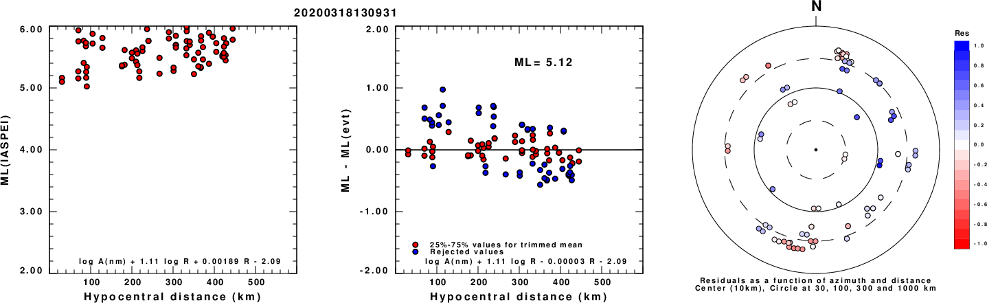
Left: ML computed using the IASPEI formula for Horizontal components. Center: ML residuals computed using a modified IASPEI formula that accounts for path specific attenuation; the values used for the trimmed mean are indicated. The ML relation used for each figure is given at the bottom of each plot. Right: Residuals from new relation as a function of distance and azimuth.

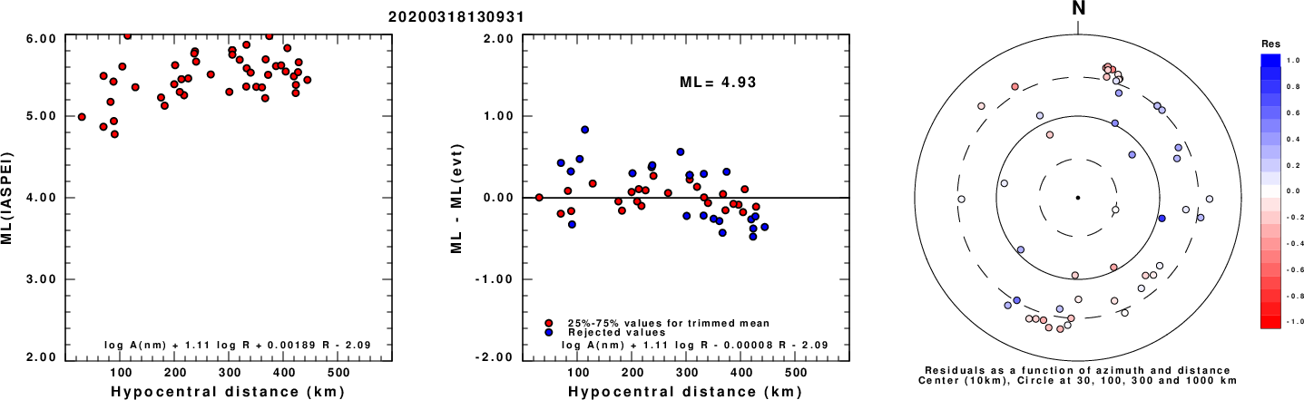
Left: ML computed using the IASPEI formula for Vertical components (research). Center: ML residuals computed using a modified IASPEI formula that accounts for path specific attenuation; the values used for the trimmed mean are indicated. The ML relation used for each figure is given at the bottom of each plot. Right: Residuals from new relation as a function of distance and azimuth.

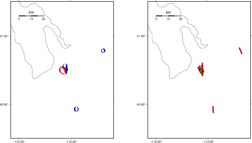
Context

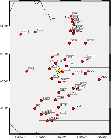
Waveform Inversion using wvfgrd96

The focal mechanism was determined using broadband seismic waveforms. The location of the event (star) and the stations used for (red) the waveform inversion are shown in the next figure.

Location of broadband stations used for waveform inversion

The program wvfgrd96 was used with good traces observed at short distance to determine the focal mechanism, depth and seismic moment. This technique requires a high quality signal and well determined velocity model for the Green's functions. To the extent that these are the quality data, this type of mechanism should be preferred over the radiation pattern technique which requires the separate step of defining the pressure and tension quadrants and the correct strike.

The observed and predicted traces are filtered using the following gsac commands:

cut o DIST/3.3 -40 o DIST/3.3 +50
rtr
taper w 0.1
hp c 0.03 n 3 
lp c 0.10 n 3 

           DEPTH  STK   DIP  RAKE   MW    FIT
WVFGRD96    1.0    75    45    85   4.99 0.1951
WVFGRD96    2.0   145    45   -90   5.16 0.2713
WVFGRD96    3.0    35    40     0   5.16 0.2513
WVFGRD96    4.0   190    25   -40   5.24 0.3186
WVFGRD96    5.0   180    25   -55   5.27 0.3989
WVFGRD96    6.0   185    30   -55   5.30 0.4658
WVFGRD96    7.0   180    30   -60   5.32 0.5226
WVFGRD96    8.0   175    30   -65   5.41 0.5695
WVFGRD96    9.0   170    30   -70   5.43 0.6116
WVFGRD96   10.0   180    35   -60   5.45 0.6409
WVFGRD96   11.0   175    35   -70   5.46 0.6582
WVFGRD96   12.0   180    35   -60   5.47 0.6650
WVFGRD96   13.0   180    35   -60   5.49 0.6640
WVFGRD96   14.0   185    40   -55   5.50 0.6574
WVFGRD96   15.0   185    40   -55   5.51 0.6449
WVFGRD96   16.0   185    40   -50   5.52 0.6281
WVFGRD96   17.0   190    45   -45   5.53 0.6089
WVFGRD96   18.0   190    45   -45   5.53 0.5879
WVFGRD96   19.0   190    45   -45   5.54 0.5639
WVFGRD96   20.0   195    50   -35   5.55 0.5383
WVFGRD96   21.0   185    30   -50   5.56 0.5160
WVFGRD96   22.0   180    30   -55   5.56 0.4921
WVFGRD96   23.0   190    35   -40   5.57 0.4686
WVFGRD96   24.0   190    35   -40   5.57 0.4450
WVFGRD96   25.0   195    35   -30   5.58 0.4225
WVFGRD96   26.0   195    35   -30   5.58 0.4004
WVFGRD96   27.0   195    40   -30   5.58 0.3799
WVFGRD96   28.0   200    35   -25   5.59 0.3648
WVFGRD96   29.0   200    35   -25   5.59 0.3519

The best solution is

WVFGRD96   12.0   180    35   -60   5.47 0.6650

The mechanism corresponding to the best fit is

Figure 1. Waveform inversion focal mechanism

The best fit as a function of depth is given in the following figure:

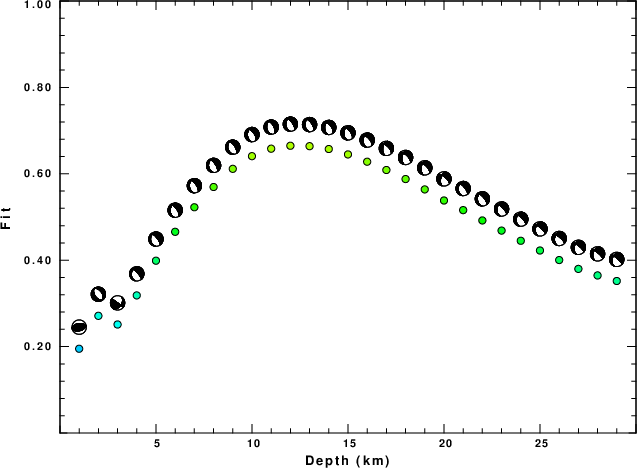
Figure 2. Depth sensitivity for waveform mechanism

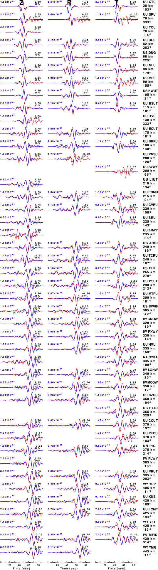
The comparison of the observed and predicted waveforms is given in the next figure. The red traces are the observed and the blue are the predicted. Each observed-predicted component is plotted to the same scale and peak amplitudes are indicated by the numbers to the left of each trace. A pair of numbers is given in black at the right of each predicted traces. The upper number it the time shift required for maximum correlation between the observed and predicted traces. This time shift is required because the synthetics are not computed at exactly the same distance as the observed, the velocity model used in the predictions may not be perfect and the epicentral parameters may be be off. A positive time shift indicates that the prediction is too fast and should be delayed to match the observed trace (shift to the right in this figure). A negative value indicates that the prediction is too slow. The lower number gives the percentage of variance reduction to characterize the individual goodness of fit (100% indicates a perfect fit).

The bandpass filter used in the processing and for the display was

cut o DIST/3.3 -40 o DIST/3.3 +50
rtr
taper w 0.1
hp c 0.03 n 3 
lp c 0.10 n 3 

Figure 3. Waveform comparison for selected depth. Red: observed; Blue - predicted. The time shift with respect to the model prediction is indicated. The percent of fit is also indicated. The time scale is relative to the first trace sample.

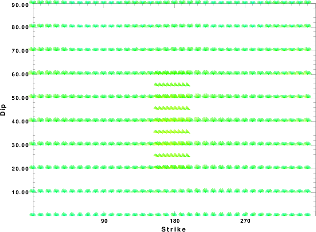
Focal mechanism sensitivity at the preferred depth. The red color indicates a very good fit to the waveforms. Each solution is plotted as a vector at a given value of strike and dip with the angle of the vector representing the rake angle, measured, with respect to the upward vertical (N) in the figure.

A check on the assumed source location is possible by looking at the time shifts between the observed and predicted traces. The time shifts for waveform matching arise for several reasons:

• The origin time and epicentral distance are incorrect
• The velocity model used for the inversion is incorrect
• The velocity model used to define the P-arrival time is not the same as the velocity model used for the waveform inversion (assuming that the initial trace alignment is based on the P arrival time)

 Time_shift = A + B cos Azimuth + C Sin Azimuth

The time shifts for this inversion lead to the next figure:

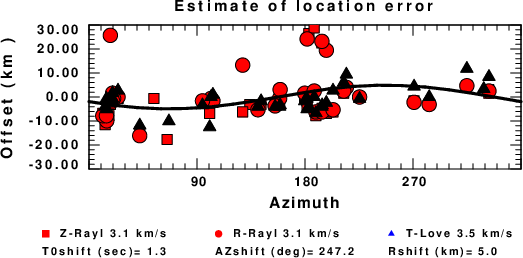
The derived shift in origin time and epicentral coordinates are given at the bottom of the figure.

Velocity Model

The WUS.model used for the waveform synthetic seismograms and for the surface wave eigenfunctions and dispersion is as follows (The format is in the model96 format of Computer Programs in Seismology).

MODEL.01
Model after     8 iterations
ISOTROPIC
KGS
FLAT EARTH
1-D
CONSTANT VELOCITY
LINE08
LINE09
LINE10
LINE11
      H(KM)   VP(KM/S)   VS(KM/S) RHO(GM/CC)         QP         QS       ETAP       ETAS      FREFP      FREFS
     1.9000     3.4065     2.0089     2.2150  0.302E-02  0.679E-02   0.00       0.00       1.00       1.00    
     6.1000     5.5445     3.2953     2.6089  0.349E-02  0.784E-02   0.00       0.00       1.00       1.00    
    13.0000     6.2708     3.7396     2.7812  0.212E-02  0.476E-02   0.00       0.00       1.00       1.00    
    19.0000     6.4075     3.7680     2.8223  0.111E-02  0.249E-02   0.00       0.00       1.00       1.00    
     0.0000     7.9000     4.6200     3.2760  0.164E-10  0.370E-10   0.00       0.00       1.00       1.00