Location
Location ANSS
The ANSS event ID is uw61562126 and the event page is at
https://earthquake.usgs.gov/earthquakes/eventpage/uw61562126/executive.
2019/11/30 01:45:12 42.776 -124.477 16.6 4.53 Oregon
Focal Mechanism
 USGS/SLU Moment Tensor Solution
 ENS  2019/11/30 01:45:12:0  42.78 -124.48  16.6 4.5 Oregon

 Stations used:
   BK.BRIC BK.DANT BK.HATC BK.PETY BK.SCOT BK.TRIN CC.CLBH
   CC.JRO CC.PRLK CC.SWNB CC.WIFE IU.COR NC.KBO NC.KHBB
   NC.KHMB NC.KMR NC.KSXB NC.LDH NC.LMC UO.BEER UO.BUCK
   UO.CAVE UO.CHIL UO.DFAZ UO.DING UO.DRAN UO.FHAC UO.JESE
   UO.LAIR UO.MARQ UO.MINN UO.NATH UO.PINE UO.ROGE UO.TOOM
   UO.VERN UO.WLOO UO.WOOD UO.WYLD UW.BBO UW.BLOW UW.HOOD
   UW.IZEE UW.LCCR UW.LEBA UW.TREE

 Filtering commands used:
   cut o DIST/3.3 -40 o DIST/3.3 +50
   rtr
   taper w 0.1
   hp c 0.03 n 3
   lp c 0.10 n 3

 Best Fitting Double Couple
  Mo = 5.96e+22 dyne-cm
  Mw = 4.45
  Z  = 18 km
  Plane   Strike  Dip  Rake
   NP1      161    86   115
   NP2      260    25    10
  Principal Axes:
   Axis    Value   Plunge  Azimuth
    T   5.96e+22     44      95
    N   0.00e+00     25     339
    P  -5.96e+22     36     229

 Moment Tensor: (dyne-cm)
    Component   Value
       Mxx    -1.62e+22
       Mxy    -2.19e+22
       Mxz     1.58e+22
       Myy     8.24e+21
       Myz     5.12e+22
       Mzz     7.92e+21


                     --------------
                 #####-----------------
              ########-----#####----------
             #######---###############-----
           ######------###################---
          ####----------####################--
         ###------------######################-
        ###--------------######################-
        ##---------------#######################
       ##-----------------#######################
       #-------------------###########   ########
       #-------------------########### T ########
       #--------------------##########   ########
        --------------------####################
        --------   ----------###################
         ------- P -----------#################
          ------   ------------###############
           --------------------##############
             -------------------###########
              -------------------#########
                 -----------------#####
                     --------------


 Global CMT Convention Moment Tensor:
      R          T          P
  7.92e+21   1.58e+22  -5.12e+22
  1.58e+22  -1.62e+22   2.19e+22
 -5.12e+22   2.19e+22   8.24e+21


Details of the solution is found at

http://www.eas.slu.edu/eqc/eqc_mt/MECH.NA/20191130014512/index.html
|
Preferred Solution
The preferred solution from an analysis of the surface-wave spectral amplitude radiation pattern, waveform inversion or first motion observations is
      STK = 260
      DIP = 25
     RAKE = 10
       MW = 4.45
       HS = 18.0
The NDK file is 20191130014512.ndk
The waveform inversion is preferred.
Moment Tensor Comparison
The following compares this source inversion to those provided by others. The purpose is to look for major differences and also to note slight differences that might be inherent to the processing procedure. For completeness the USGS/SLU solution is repeated from above.
| SLU |
USGSMWR |
 USGS/SLU Moment Tensor Solution
 ENS  2019/11/30 01:45:12:0  42.78 -124.48  16.6 4.5 Oregon

 Stations used:
   BK.BRIC BK.DANT BK.HATC BK.PETY BK.SCOT BK.TRIN CC.CLBH
   CC.JRO CC.PRLK CC.SWNB CC.WIFE IU.COR NC.KBO NC.KHBB
   NC.KHMB NC.KMR NC.KSXB NC.LDH NC.LMC UO.BEER UO.BUCK
   UO.CAVE UO.CHIL UO.DFAZ UO.DING UO.DRAN UO.FHAC UO.JESE
   UO.LAIR UO.MARQ UO.MINN UO.NATH UO.PINE UO.ROGE UO.TOOM
   UO.VERN UO.WLOO UO.WOOD UO.WYLD UW.BBO UW.BLOW UW.HOOD
   UW.IZEE UW.LCCR UW.LEBA UW.TREE

 Filtering commands used:
   cut o DIST/3.3 -40 o DIST/3.3 +50
   rtr
   taper w 0.1
   hp c 0.03 n 3
   lp c 0.10 n 3

 Best Fitting Double Couple
  Mo = 5.96e+22 dyne-cm
  Mw = 4.45
  Z  = 18 km
  Plane   Strike  Dip  Rake
   NP1      161    86   115
   NP2      260    25    10
  Principal Axes:
   Axis    Value   Plunge  Azimuth
    T   5.96e+22     44      95
    N   0.00e+00     25     339
    P  -5.96e+22     36     229

 Moment Tensor: (dyne-cm)
    Component   Value
       Mxx    -1.62e+22
       Mxy    -2.19e+22
       Mxz     1.58e+22
       Myy     8.24e+21
       Myz     5.12e+22
       Mzz     7.92e+21


                     --------------
                 #####-----------------
              ########-----#####----------
             #######---###############-----
           ######------###################---
          ####----------####################--
         ###------------######################-
        ###--------------######################-
        ##---------------#######################
       ##-----------------#######################
       #-------------------###########   ########
       #-------------------########### T ########
       #--------------------##########   ########
        --------------------####################
        --------   ----------###################
         ------- P -----------#################
          ------   ------------###############
           --------------------##############
             -------------------###########
              -------------------#########
                 -----------------#####
                     --------------


 Global CMT Convention Moment Tensor:
      R          T          P
  7.92e+21   1.58e+22  -5.12e+22
  1.58e+22  -1.62e+22   2.19e+22
 -5.12e+22   2.19e+22   8.24e+21


Details of the solution is found at

http://www.eas.slu.edu/eqc/eqc_mt/MECH.NA/20191130014512/index.html
|
Regional Moment Tensor (Mwr)
Moment 6.802e+15 N-m
Magnitude 4.49 Mwr
Depth 21.0 km
Percent DC 91%
Half Duration -
Catalog US
Data Source US 3
Contributor US 3
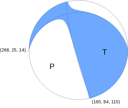
Nodal Planes
Plane Strike Dip Rake
NP1 268� 25� 14�
NP2 165� 84� 115�
Principal Axes
Axis Value Plunge Azimuth
T 6.646e+15 N-m 46� 100�
N 0.303e+15 N-m 25� 342�
P -6.949e+15 N-m 34� 234�
 |
Magnitudes
Given the availability of digital waveforms for determination of the moment tensor, this section documents the added processing leading to mLg, if appropriate to the region, and ML by application of the respective IASPEI formulae. As a research study, the linear distance term of the IASPEI formula
for ML is adjusted to remove a linear distance trend in residuals to give a regionally defined ML. The defined ML uses horizontal component recordings, but the same procedure is applied to the vertical components since there may be some interest in vertical component ground motions. Residual plots versus distance may indicate interesting features of ground motion scaling in some distance ranges. A residual plot of the regionalized magnitude is given as a function of distance and azimuth, since data sets may transcend different wave propagation provinces.
mLg Magnitude
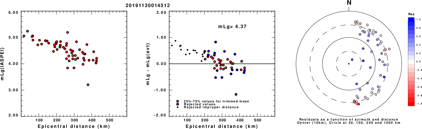
Left: mLg computed using the IASPEI formula. Center: mLg residuals versus epicentral distance ; the values used for the trimmed mean magnitude estimate are indicated.
Right: residuals as a function of distance and azimuth.
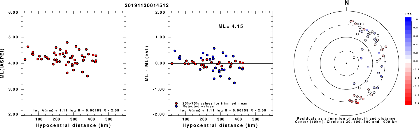
ML Magnitude
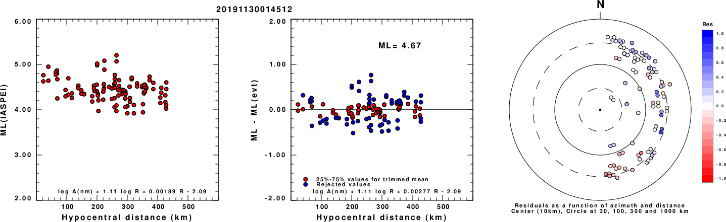
Left: ML computed using the IASPEI formula for Horizontal components. Center: ML residuals computed using a modified IASPEI formula that accounts for path specific attenuation; the values used for the trimmed mean are indicated. The ML relation used for each figure is given at the bottom of each plot.
Right: Residuals from new relation as a function of distance and azimuth.
Left: ML computed using the IASPEI formula for Vertical components (research). Center: ML residuals computed using a modified IASPEI formula that accounts for path specific attenuation; the values used for the trimmed mean are indicated. The ML relation used for each figure is given at the bottom of each plot.
Right: Residuals from new relation as a function of distance and azimuth.
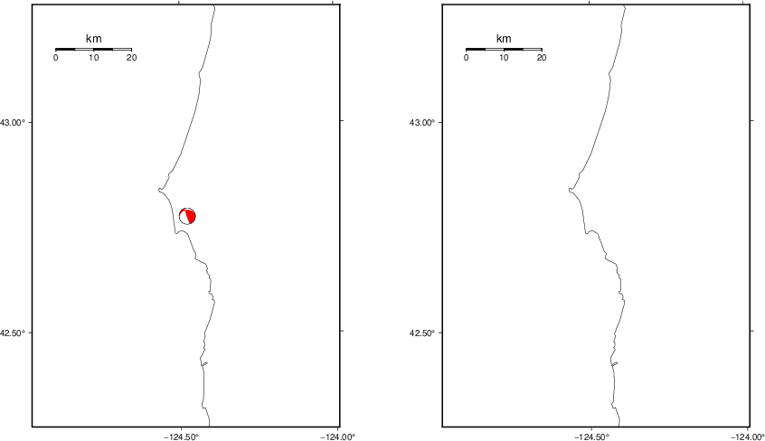
Context
The left panel of the next figure presents the focal mechanism for this earthquake (red) in the context of other nearby events (blue) in the SLU Moment Tensor Catalog. The right panel shows the inferred direction of maximum compressive stress and the type of faulting (green is strike-slip, red is normal, blue is thrust; oblique is shown by a combination of colors). Thus context plot is useful for assessing the appropriateness of the moment tensor of this event.
Waveform Inversion using wvfgrd96
The focal mechanism was determined using broadband seismic waveforms. The location of the event (star) and the
stations used for (red) the waveform inversion are shown in the next figure.

|
|
Location of broadband stations used for waveform inversion
|
The program wvfgrd96 was used with good traces observed at short distance to determine the focal mechanism, depth and seismic moment. This technique requires a high quality signal and well determined velocity model for the Green's functions. To the extent that these are the quality data, this type of mechanism should be preferred over the radiation pattern technique which requires the separate step of defining the pressure and tension quadrants and the correct strike.
The observed and predicted traces are filtered using the following gsac commands:
cut o DIST/3.3 -40 o DIST/3.3 +50
rtr
taper w 0.1
hp c 0.03 n 3
lp c 0.10 n 3
The results of this grid search are as follow:
           DEPTH  STK   DIP  RAKE   MW    FIT
WVFGRD96    1.0   330    45   -90   4.00 0.2674
WVFGRD96    2.0   150    45   -90   4.16 0.3550
WVFGRD96    3.0   325    40   -95   4.18 0.2484
WVFGRD96    4.0   340    85   -65   4.13 0.2333
WVFGRD96    5.0   160    90    65   4.15 0.2933
WVFGRD96    6.0   160    90    65   4.18 0.3493
WVFGRD96    7.0   160    90    65   4.19 0.3960
WVFGRD96    8.0   340    90   -65   4.28 0.4300
WVFGRD96    9.0   160    90    65   4.30 0.4726
WVFGRD96   10.0   160    85    65   4.32 0.5098
WVFGRD96   11.0   335    90   -65   4.34 0.5396
WVFGRD96   12.0   160    85    65   4.36 0.5675
WVFGRD96   13.0   160    85    65   4.38 0.5883
WVFGRD96   14.0   265    25    15   4.39 0.6026
WVFGRD96   15.0   260    25    10   4.41 0.6162
WVFGRD96   16.0   260    25    10   4.43 0.6251
WVFGRD96   17.0   260    25    10   4.44 0.6304
WVFGRD96   18.0   260    25    10   4.45 0.6322
WVFGRD96   19.0   260    25    10   4.47 0.6308
WVFGRD96   20.0   260    25    10   4.48 0.6264
WVFGRD96   21.0   260    25    10   4.50 0.6198
WVFGRD96   22.0   260    25    10   4.51 0.6103
WVFGRD96   23.0   260    25    10   4.52 0.5989
WVFGRD96   24.0   265    25    15   4.53 0.5853
WVFGRD96   25.0   265    25    15   4.54 0.5700
WVFGRD96   26.0   315    40    70   4.56 0.5543
WVFGRD96   27.0   315    40    70   4.57 0.5388
WVFGRD96   28.0   310    40    60   4.58 0.5230
WVFGRD96   29.0   305    40    55   4.58 0.5065
The best solution is
WVFGRD96 18.0 260 25 10 4.45 0.6322
The mechanism corresponding to the best fit is
|
|
Figure 1. Waveform inversion focal mechanism
|
The best fit as a function of depth is given in the following figure:
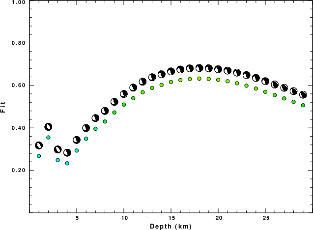
|
|
Figure 2. Depth sensitivity for waveform mechanism
|
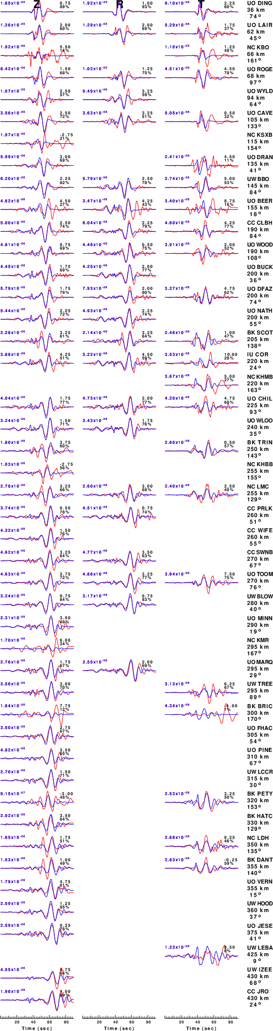
The comparison of the observed and predicted waveforms is given in the next figure. The red traces are the observed and the blue are the predicted.
Each observed-predicted component is plotted to the same scale and peak amplitudes are indicated by the numbers to the left of each trace. A pair of numbers is given in black at the right of each predicted traces. The upper number it the time shift required for maximum correlation between the observed and predicted traces. This time shift is required because the synthetics are not computed at exactly the same distance as the observed, the velocity model used in the predictions may not be perfect and the epicentral parameters may be be off.
A positive time shift indicates that the prediction is too fast and should be delayed to match the observed trace (shift to the right in this figure). A negative value indicates that the prediction is too slow. The lower number gives the percentage of variance reduction to characterize the individual goodness of fit (100% indicates a perfect fit).
The bandpass filter used in the processing and for the display was
cut o DIST/3.3 -40 o DIST/3.3 +50
rtr
taper w 0.1
hp c 0.03 n 3
lp c 0.10 n 3
|
|
Figure 3. Waveform comparison for selected depth. Red: observed; Blue - predicted. The time shift with respect to the model prediction is indicated. The percent of fit is also indicated. The time scale is relative to the first trace sample.
|
|
|
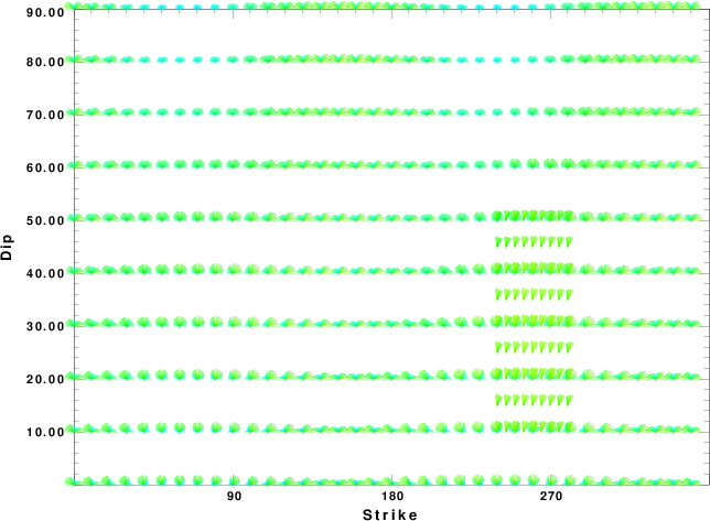
Focal mechanism sensitivity at the preferred depth. The red color indicates a very good fit to the waveforms.
Each solution is plotted as a vector at a given value of strike and dip with the angle of the vector representing the rake angle, measured, with respect to the upward vertical (N) in the figure.
|
A check on the assumed source location is possible by looking at the time shifts between the observed and predicted traces. The time shifts for waveform matching arise for several reasons:
- The origin time and epicentral distance are incorrect
- The velocity model used for the inversion is incorrect
- The velocity model used to define the P-arrival time is not the
same as the velocity model used for the waveform inversion
(assuming that the initial trace alignment is based on the
P arrival time)
Assuming only a mislocation, the time shifts are fit to a functional form:
Time_shift = A + B cos Azimuth + C Sin Azimuth
The time shifts for this inversion lead to the next figure:
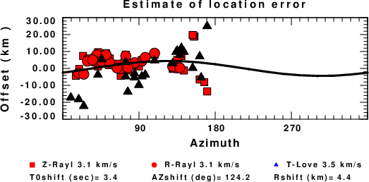
The derived shift in origin time and epicentral coordinates are given at the bottom of the figure.
Velocity Model
The WUS.model used for the waveform synthetic seismograms and for the surface wave eigenfunctions and dispersion is as follows
(The format is in the model96 format of Computer Programs in Seismology).
MODEL.01
Model after     8 iterations
ISOTROPIC
KGS
FLAT EARTH
1-D
CONSTANT VELOCITY
LINE08
LINE09
LINE10
LINE11
      H(KM)   VP(KM/S)   VS(KM/S) RHO(GM/CC)         QP         QS       ETAP       ETAS      FREFP      FREFS
     1.9000     3.4065     2.0089     2.2150  0.302E-02  0.679E-02   0.00       0.00       1.00       1.00
     6.1000     5.5445     3.2953     2.6089  0.349E-02  0.784E-02   0.00       0.00       1.00       1.00
    13.0000     6.2708     3.7396     2.7812  0.212E-02  0.476E-02   0.00       0.00       1.00       1.00
    19.0000     6.4075     3.7680     2.8223  0.111E-02  0.249E-02   0.00       0.00       1.00       1.00
     0.0000     7.9000     4.6200     3.2760  0.164E-10  0.370E-10   0.00       0.00       1.00       1.00
Last Changed Thu Apr 25 05:47:12 PM CDT 2024