Location

Location ANSS

The ANSS event ID is ak0193wxcfea and the event page is at https://earthquake.usgs.gov/earthquakes/eventpage/ak0193wxcfea/executive.

2019/03/26 21:27:19 66.306 -157.247 8.5 5 Alaska

Focal Mechanism

USGS/SLU Moment Tensor Solution ENS 2019/03/26 21:27:19:0 66.31 -157.25 8.5 5.0 Alaska Stations used: AK.ANM AK.BPAW AK.BWN AK.CAST AK.CCB AK.CHUM AK.COLD AK.CUT AK.FA01 AK.FA02 AK.GCSA AK.HDA AK.KTH AK.PPD AK.PPLA AK.RDOG AK.RND AK.SKN AK.TNA AK.TRF AV.STLK IU.COLA TA.B18K TA.C17K TA.D17K TA.D23K TA.E23K TA.E25K TA.F14K TA.F17K TA.F18K TA.F19K TA.F21K TA.F22K TA.F24K TA.F25K TA.F26K TA.G17K TA.G18K TA.G23K TA.G24K TA.G26K TA.H16K TA.H17K TA.H19K TA.H20K TA.H21K TA.H24K TA.I17K TA.I20K TA.I23K TA.J14K TA.J16K TA.J17K TA.J18K TA.J19K TA.J20K TA.J25K TA.K13K TA.K15K TA.K17K TA.L16K TA.L17K TA.L18K TA.L19K TA.L20K TA.M16K TA.M17K TA.M18K TA.M20K TA.POKR TA.TOLK XV.F1TN XV.F2TN XV.F3TN XV.F4TN XV.F6TP XV.F7TV XV.F8KN XV.FAPT XV.FNN1 XV.FNN2 XV.FPAP Filtering commands used: cut o DIST/3.3 -40 o DIST/3.3 +50 rtr taper w 0.1 hp c 0.03 n 3 lp c 0.07 n 3 Best Fitting Double Couple Mo = 3.59e+23 dyne-cm Mw = 4.97 Z = 12 km Plane Strike Dip Rake NP1 350 85 20 NP2 258 70 175 Principal Axes: Axis Value Plunge Azimuth T 3.59e+23 18 216 N 0.00e+00 69 3 P -3.59e+23 10 122 Moment Tensor: (dyne-cm) Component Value Mxx 1.14e+23 Mxy 3.12e+23 Mxz -4.99e+22 Myy -1.36e+23 Myz -1.14e+23 Mzz 2.13e+22 ----########## --------############## ------------################ -------------################# ----------------################## -----------------################### -------------------################### --------------------#################### -----------------###-------------------# ------------##########-------------------- --------##############-------------------- -----#################-------------------- --#####################------------------- ######################------------------ ######################------------------ ######################----------- -- #####################----------- P - ##### ############----------- ### T ############------------ ## ############----------- ###############------- ###########--- Global CMT Convention Moment Tensor: R T P 2.13e+22 -4.99e+22 1.14e+23 -4.99e+22 1.14e+23 -3.12e+23 1.14e+23 -3.12e+23 -1.36e+23 Details of the solution is found at http://www.eas.slu.edu/eqc/eqc_mt/MECH.NA/20190326212719/index.html

Preferred Solution

      STK = 350
      DIP = 85
     RAKE = 20
       MW = 4.97
       HS = 12.0

The NDK file is 20190326212719.ndk The waveform inversion is preferred.

Moment Tensor Comparison

The following compares this source inversion to those provided by others. The purpose is to look for major differences and also to note slight differences that might be inherent to the processing procedure. For completeness the USGS/SLU solution is repeated from above.

SLU	USGSMWR	USGSW
USGS/SLU Moment Tensor Solution ENS 2019/03/26 21:27:19:0 66.31 -157.25 8.5 5.0 Alaska Stations used: AK.ANM AK.BPAW AK.BWN AK.CAST AK.CCB AK.CHUM AK.COLD AK.CUT AK.FA01 AK.FA02 AK.GCSA AK.HDA AK.KTH AK.PPD AK.PPLA AK.RDOG AK.RND AK.SKN AK.TNA AK.TRF AV.STLK IU.COLA TA.B18K TA.C17K TA.D17K TA.D23K TA.E23K TA.E25K TA.F14K TA.F17K TA.F18K TA.F19K TA.F21K TA.F22K TA.F24K TA.F25K TA.F26K TA.G17K TA.G18K TA.G23K TA.G24K TA.G26K TA.H16K TA.H17K TA.H19K TA.H20K TA.H21K TA.H24K TA.I17K TA.I20K TA.I23K TA.J14K TA.J16K TA.J17K TA.J18K TA.J19K TA.J20K TA.J25K TA.K13K TA.K15K TA.K17K TA.L16K TA.L17K TA.L18K TA.L19K TA.L20K TA.M16K TA.M17K TA.M18K TA.M20K TA.POKR TA.TOLK XV.F1TN XV.F2TN XV.F3TN XV.F4TN XV.F6TP XV.F7TV XV.F8KN XV.FAPT XV.FNN1 XV.FNN2 XV.FPAP Filtering commands used: cut o DIST/3.3 -40 o DIST/3.3 +50 rtr taper w 0.1 hp c 0.03 n 3 lp c 0.07 n 3 Best Fitting Double Couple Mo = 3.59e+23 dyne-cm Mw = 4.97 Z = 12 km Plane Strike Dip Rake NP1 350 85 20 NP2 258 70 175 Principal Axes: Axis Value Plunge Azimuth T 3.59e+23 18 216 N 0.00e+00 69 3 P -3.59e+23 10 122 Moment Tensor: (dyne-cm) Component Value Mxx 1.14e+23 Mxy 3.12e+23 Mxz -4.99e+22 Myy -1.36e+23 Myz -1.14e+23 Mzz 2.13e+22 ----########## --------############## ------------################ -------------################# ----------------################## -----------------################### -------------------################### --------------------#################### -----------------###-------------------# ------------##########-------------------- --------##############-------------------- -----#################-------------------- --#####################------------------- ######################------------------ ######################------------------ ######################----------- -- #####################----------- P - ##### ############----------- ### T ############------------ ## ############----------- ###############------- ###########--- Global CMT Convention Moment Tensor: R T P 2.13e+22 -4.99e+22 1.14e+23 -4.99e+22 1.14e+23 -3.12e+23 1.14e+23 -3.12e+23 -1.36e+23 Details of the solution is found at http://www.eas.slu.edu/eqc/eqc_mt/MECH.NA/20190326212719/index.html	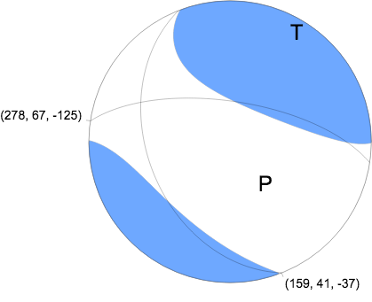egional Moment Tensor (Mwr) Moment 3.085e+16 N-m Magnitude 4.93 Mwr Depth 5.0 km Percent DC 37% Half Duration - Catalog US Data Source US 2 Contributor US 2 Nodal Planes Plane Strike Dip Rake NP1 159 41 -37 NP2 278 67 -125 Principal Axes Axis Value Plunge Azimuth T 3.482e+16 N-m 15 33 N -1.092e+16 N-m 31 294 P -2.390e+16 N-m 55 145	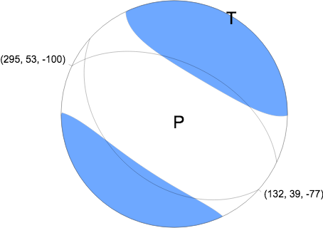W-phase Moment Tensor (Mww) Moment 4.616e+16 N-m Magnitude 5.04 Mww Depth 11.5 km Percent DC 25% Half Duration 0.84 s Catalog US Data Source US 2 Contributor US 2 Nodal Planes Plane Strike Dip Rake NP1 132 39 -77 NP2 295 53 -100 Principal Axes Axis Value Plunge Azimuth T 5.276e+16 N-m 7 32 N -1.982e+16 N-m 8 301 P -3.294e+16 N-m 79 163

Magnitudes

Given the availability of digital waveforms for determination of the moment tensor, this section documents the added processing leading to mLg, if appropriate to the region, and M_L by application of the respective IASPEI formulae. As a research study, the linear distance term of the IASPEI formula for M_L is adjusted to remove a linear distance trend in residuals to give a regionally defined M_L. The defined M_L uses horizontal component recordings, but the same procedure is applied to the vertical components since there may be some interest in vertical component ground motions. Residual plots versus distance may indicate interesting features of ground motion scaling in some distance ranges. A residual plot of the regionalized magnitude is given as a function of distance and azimuth, since data sets may transcend different wave propagation provinces.

mLg Magnitude

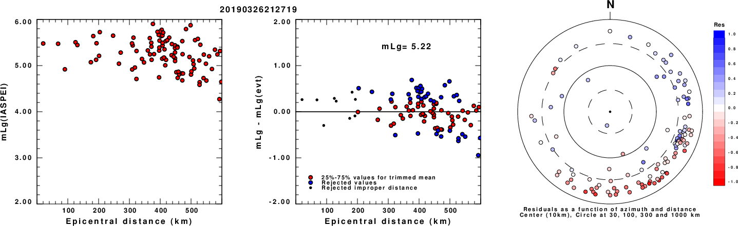
Left: mLg computed using the IASPEI formula. Center: mLg residuals versus epicentral distance ; the values used for the trimmed mean magnitude estimate are indicated. Right: residuals as a function of distance and azimuth.

ML Magnitude

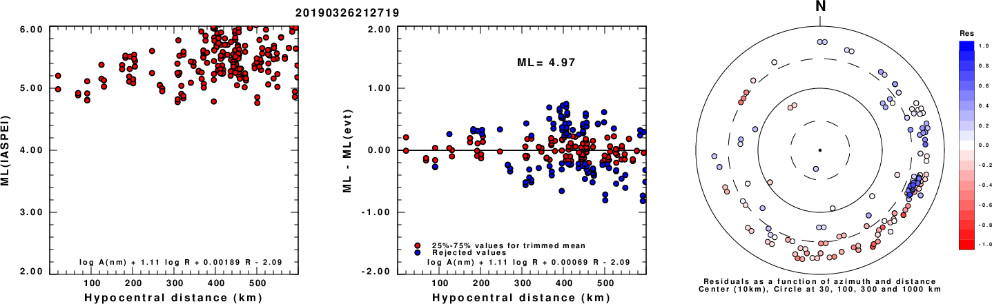
Left: ML computed using the IASPEI formula for Horizontal components. Center: ML residuals computed using a modified IASPEI formula that accounts for path specific attenuation; the values used for the trimmed mean are indicated. The ML relation used for each figure is given at the bottom of each plot. Right: Residuals from new relation as a function of distance and azimuth.

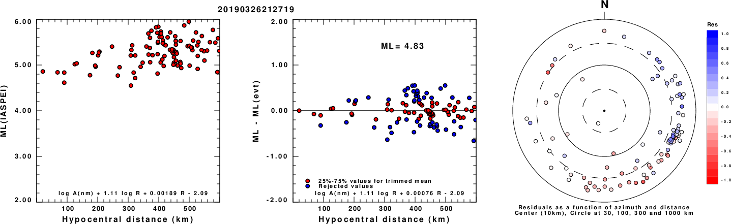
Left: ML computed using the IASPEI formula for Vertical components (research). Center: ML residuals computed using a modified IASPEI formula that accounts for path specific attenuation; the values used for the trimmed mean are indicated. The ML relation used for each figure is given at the bottom of each plot. Right: Residuals from new relation as a function of distance and azimuth.

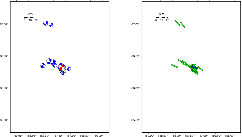
Context

Waveform Inversion using wvfgrd96

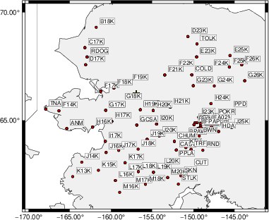
The focal mechanism was determined using broadband seismic waveforms. The location of the event (star) and the stations used for (red) the waveform inversion are shown in the next figure.

Location of broadband stations used for waveform inversion

The program wvfgrd96 was used with good traces observed at short distance to determine the focal mechanism, depth and seismic moment. This technique requires a high quality signal and well determined velocity model for the Green's functions. To the extent that these are the quality data, this type of mechanism should be preferred over the radiation pattern technique which requires the separate step of defining the pressure and tension quadrants and the correct strike.

The observed and predicted traces are filtered using the following gsac commands:

cut o DIST/3.3 -40 o DIST/3.3 +50
rtr
taper w 0.1
hp c 0.03 n 3 
lp c 0.07 n 3 

           DEPTH  STK   DIP  RAKE   MW    FIT
WVFGRD96    1.0   350    75   -15   4.62 0.4195
WVFGRD96    2.0   345    65   -25   4.75 0.5384
WVFGRD96    3.0   345    65   -25   4.80 0.5815
WVFGRD96    4.0   350    75   -15   4.81 0.6049
WVFGRD96    5.0   350    80   -15   4.83 0.6187
WVFGRD96    6.0   165    75   -25   4.86 0.6348
WVFGRD96    7.0   170    85   -20   4.88 0.6497
WVFGRD96    8.0   165    75   -30   4.92 0.6691
WVFGRD96    9.0   170    85   -25   4.93 0.6728
WVFGRD96   10.0   350    90    25   4.95 0.6727
WVFGRD96   11.0   350    85    20   4.96 0.6749
WVFGRD96   12.0   350    85    20   4.97 0.6750
WVFGRD96   13.0   350    85    20   4.98 0.6714
WVFGRD96   14.0   350    85    20   4.99 0.6655
WVFGRD96   15.0   350    80    20   5.00 0.6575
WVFGRD96   16.0   350    80    15   5.01 0.6484
WVFGRD96   17.0   350    80    15   5.02 0.6388
WVFGRD96   18.0   350    80    15   5.02 0.6285
WVFGRD96   19.0   350    80    15   5.03 0.6176
WVFGRD96   20.0   350    80    15   5.04 0.6064
WVFGRD96   21.0   350    80    15   5.04 0.5949
WVFGRD96   22.0   350    80    15   5.05 0.5840
WVFGRD96   23.0   350    80    15   5.05 0.5729
WVFGRD96   24.0   350    80    15   5.06 0.5616
WVFGRD96   25.0   350    80    15   5.07 0.5500
WVFGRD96   26.0   350    80    15   5.07 0.5383
WVFGRD96   27.0   350    80    15   5.08 0.5268
WVFGRD96   28.0   350    75    10   5.08 0.5153
WVFGRD96   29.0   350    75    10   5.09 0.5038

The best solution is

WVFGRD96   12.0   350    85    20   4.97 0.6750

The mechanism corresponding to the best fit is

Figure 1. Waveform inversion focal mechanism

The best fit as a function of depth is given in the following figure:

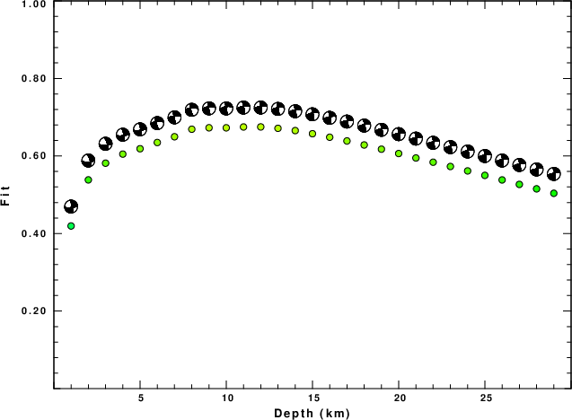
Figure 2. Depth sensitivity for waveform mechanism

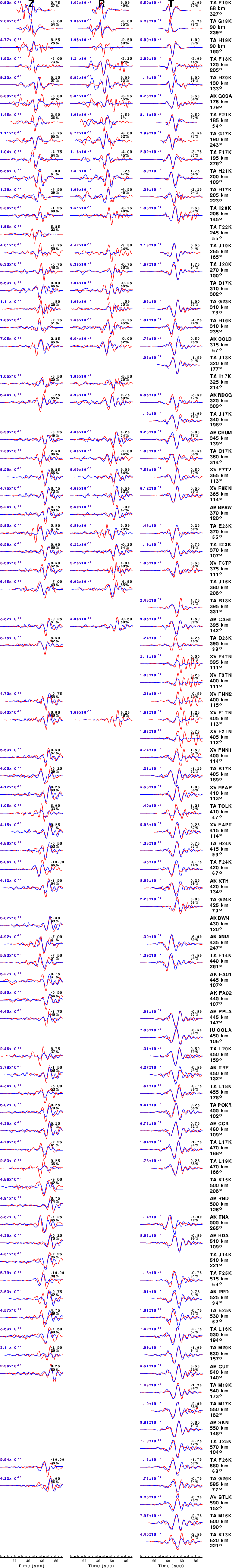
The comparison of the observed and predicted waveforms is given in the next figure. The red traces are the observed and the blue are the predicted. Each observed-predicted component is plotted to the same scale and peak amplitudes are indicated by the numbers to the left of each trace. A pair of numbers is given in black at the right of each predicted traces. The upper number it the time shift required for maximum correlation between the observed and predicted traces. This time shift is required because the synthetics are not computed at exactly the same distance as the observed, the velocity model used in the predictions may not be perfect and the epicentral parameters may be be off. A positive time shift indicates that the prediction is too fast and should be delayed to match the observed trace (shift to the right in this figure). A negative value indicates that the prediction is too slow. The lower number gives the percentage of variance reduction to characterize the individual goodness of fit (100% indicates a perfect fit).

The bandpass filter used in the processing and for the display was

cut o DIST/3.3 -40 o DIST/3.3 +50
rtr
taper w 0.1
hp c 0.03 n 3 
lp c 0.07 n 3 

Figure 3. Waveform comparison for selected depth. Red: observed; Blue - predicted. The time shift with respect to the model prediction is indicated. The percent of fit is also indicated. The time scale is relative to the first trace sample.

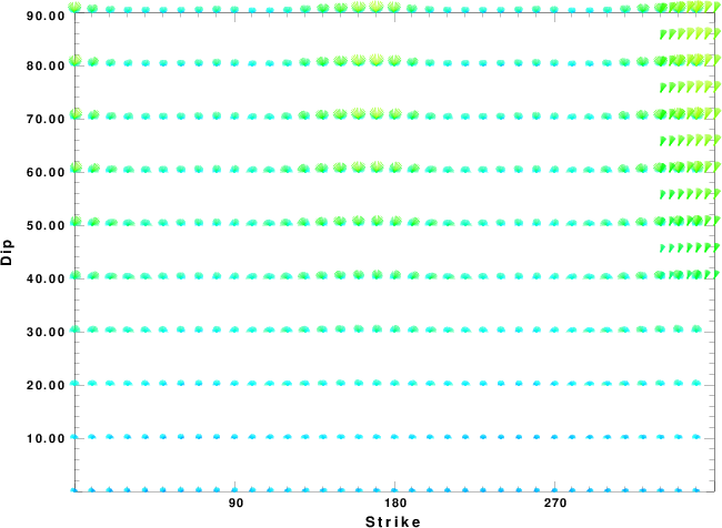
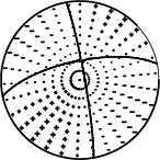
Focal mechanism sensitivity at the preferred depth. The red color indicates a very good fit to the waveforms. Each solution is plotted as a vector at a given value of strike and dip with the angle of the vector representing the rake angle, measured, with respect to the upward vertical (N) in the figure.

A check on the assumed source location is possible by looking at the time shifts between the observed and predicted traces. The time shifts for waveform matching arise for several reasons:

• The origin time and epicentral distance are incorrect
• The velocity model used for the inversion is incorrect
• The velocity model used to define the P-arrival time is not the same as the velocity model used for the waveform inversion (assuming that the initial trace alignment is based on the P arrival time)

 Time_shift = A + B cos Azimuth + C Sin Azimuth

The time shifts for this inversion lead to the next figure:

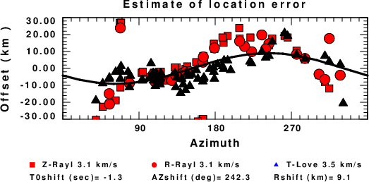
The derived shift in origin time and epicentral coordinates are given at the bottom of the figure.

Velocity Model

The WUS.model used for the waveform synthetic seismograms and for the surface wave eigenfunctions and dispersion is as follows (The format is in the model96 format of Computer Programs in Seismology).

MODEL.01
Model after     8 iterations
ISOTROPIC
KGS
FLAT EARTH
1-D
CONSTANT VELOCITY
LINE08
LINE09
LINE10
LINE11
      H(KM)   VP(KM/S)   VS(KM/S) RHO(GM/CC)         QP         QS       ETAP       ETAS      FREFP      FREFS
     1.9000     3.4065     2.0089     2.2150  0.302E-02  0.679E-02   0.00       0.00       1.00       1.00    
     6.1000     5.5445     3.2953     2.6089  0.349E-02  0.784E-02   0.00       0.00       1.00       1.00    
    13.0000     6.2708     3.7396     2.7812  0.212E-02  0.476E-02   0.00       0.00       1.00       1.00    
    19.0000     6.4075     3.7680     2.8223  0.111E-02  0.249E-02   0.00       0.00       1.00       1.00    
     0.0000     7.9000     4.6200     3.2760  0.164E-10  0.370E-10   0.00       0.00       1.00       1.00