Location
SLU Location
To check the ANSS location or to compare the observed P-wave first motions to the moment tensor solution, P- and S-wave first arrival times were manually read together with the P-wave first motions. The subsequent output of the program elocate is given in the file elocate.txt. The first motion plot is shown below.
Location ANSS
The ANSS event ID is ak0193rv320m and the event page is at
https://earthquake.usgs.gov/earthquakes/eventpage/ak0193rv320m/executive.
2019/03/23 15:14:44 61.526 -149.862 47.4 4.1 Alaska
Focal Mechanism
 USGS/SLU Moment Tensor Solution
 ENS  2019/03/23 15:14:44:0  61.53 -149.86  47.4 4.1 Alaska

 Stations used:
   AK.CUT AK.GHO AK.KLU AK.KNK AK.PWL AK.RC01 AK.SAW AK.SCM
   AK.SLK AK.SWD AT.PMR AV.STLK GM.AD09 TA.M23K TA.M24K
   TA.O22K TA.P19K

 Filtering commands used:
   cut o DIST/3.3 -40 o DIST/3.3 +50
   rtr
   taper w 0.1
   hp c 0.03 n 3
   lp c 0.08 n 3

 Best Fitting Double Couple
  Mo = 2.04e+22 dyne-cm
  Mw = 4.14
  Z  = 49 km
  Plane   Strike  Dip  Rake
   NP1      230    55   -50
   NP2      354    51   -133
  Principal Axes:
   Axis    Value   Plunge  Azimuth
    T   2.04e+22      2     293
    N   0.00e+00     32      24
    P  -2.04e+22     58     199

 Moment Tensor: (dyne-cm)
    Component   Value
       Mxx    -1.96e+21
       Mxy    -9.10e+21
       Mxz     8.94e+21
       Myy     1.67e+22
       Myz     2.33e+21
       Mzz    -1.47e+22


                     #######-------
                 #############---------
              ##################----------
             ####################----------
           ####################---###########
           ################--------###########
         T #############------------###########
           ###########---------------###########
        ############-----------------###########
       ###########-------------------############
       ##########---------------------###########
       #########----------------------###########
       ########-----------------------###########
        ######------------------------##########
        #####-----------   -----------##########
         ###------------ P ----------##########
          ##------------   ----------#########
           #------------------------#########
             ----------------------########
              --------------------########
                 ----------------######
                     ----------####


 Global CMT Convention Moment Tensor:
      R          T          P
 -1.47e+22   8.94e+21  -2.33e+21
  8.94e+21  -1.96e+21   9.10e+21
 -2.33e+21   9.10e+21   1.67e+22


Details of the solution is found at

http://www.eas.slu.edu/eqc/eqc_mt/MECH.NA/20190323151444/index.html
|
Preferred Solution
The preferred solution from an analysis of the surface-wave spectral amplitude radiation pattern, waveform inversion or first motion observations is
      STK = 230
      DIP = 55
     RAKE = -50
       MW = 4.14
       HS = 49.0
The NDK file is 20190323151444.ndk
The waveform inversion is preferred.
Moment Tensor Comparison
The following compares this source inversion to those provided by others. The purpose is to look for major differences and also to note slight differences that might be inherent to the processing procedure. For completeness the USGS/SLU solution is repeated from above.
| SLU |
SLUFM |
 USGS/SLU Moment Tensor Solution
 ENS  2019/03/23 15:14:44:0  61.53 -149.86  47.4 4.1 Alaska

 Stations used:
   AK.CUT AK.GHO AK.KLU AK.KNK AK.PWL AK.RC01 AK.SAW AK.SCM
   AK.SLK AK.SWD AT.PMR AV.STLK GM.AD09 TA.M23K TA.M24K
   TA.O22K TA.P19K

 Filtering commands used:
   cut o DIST/3.3 -40 o DIST/3.3 +50
   rtr
   taper w 0.1
   hp c 0.03 n 3
   lp c 0.08 n 3

 Best Fitting Double Couple
  Mo = 2.04e+22 dyne-cm
  Mw = 4.14
  Z  = 49 km
  Plane   Strike  Dip  Rake
   NP1      230    55   -50
   NP2      354    51   -133
  Principal Axes:
   Axis    Value   Plunge  Azimuth
    T   2.04e+22      2     293
    N   0.00e+00     32      24
    P  -2.04e+22     58     199

 Moment Tensor: (dyne-cm)
    Component   Value
       Mxx    -1.96e+21
       Mxy    -9.10e+21
       Mxz     8.94e+21
       Myy     1.67e+22
       Myz     2.33e+21
       Mzz    -1.47e+22


                     #######-------
                 #############---------
              ##################----------
             ####################----------
           ####################---###########
           ################--------###########
         T #############------------###########
           ###########---------------###########
        ############-----------------###########
       ###########-------------------############
       ##########---------------------###########
       #########----------------------###########
       ########-----------------------###########
        ######------------------------##########
        #####-----------   -----------##########
         ###------------ P ----------##########
          ##------------   ----------#########
           #------------------------#########
             ----------------------########
              --------------------########
                 ----------------######
                     ----------####


 Global CMT Convention Moment Tensor:
      R          T          P
 -1.47e+22   8.94e+21  -2.33e+21
  8.94e+21  -1.96e+21   9.10e+21
 -2.33e+21   9.10e+21   1.67e+22


Details of the solution is found at

http://www.eas.slu.edu/eqc/eqc_mt/MECH.NA/20190323151444/index.html
|
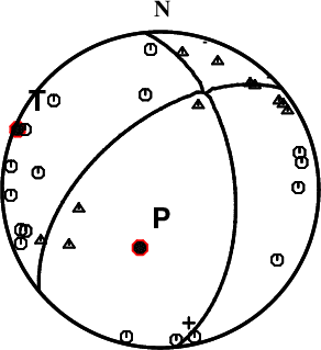
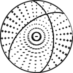
First motions and takeoff angles from an elocate run.
|
Magnitudes
Given the availability of digital waveforms for determination of the moment tensor, this section documents the added processing leading to mLg, if appropriate to the region, and ML by application of the respective IASPEI formulae. As a research study, the linear distance term of the IASPEI formula
for ML is adjusted to remove a linear distance trend in residuals to give a regionally defined ML. The defined ML uses horizontal component recordings, but the same procedure is applied to the vertical components since there may be some interest in vertical component ground motions. Residual plots versus distance may indicate interesting features of ground motion scaling in some distance ranges. A residual plot of the regionalized magnitude is given as a function of distance and azimuth, since data sets may transcend different wave propagation provinces.
mLg Magnitude
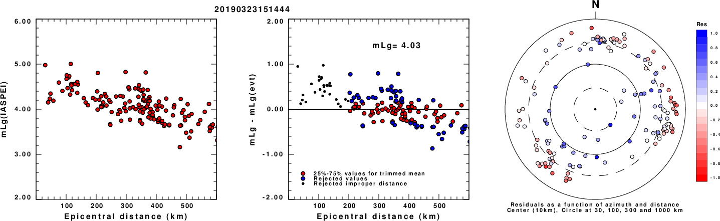
Left: mLg computed using the IASPEI formula. Center: mLg residuals versus epicentral distance ; the values used for the trimmed mean magnitude estimate are indicated.
Right: residuals as a function of distance and azimuth.
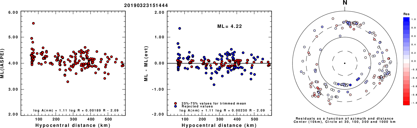
ML Magnitude
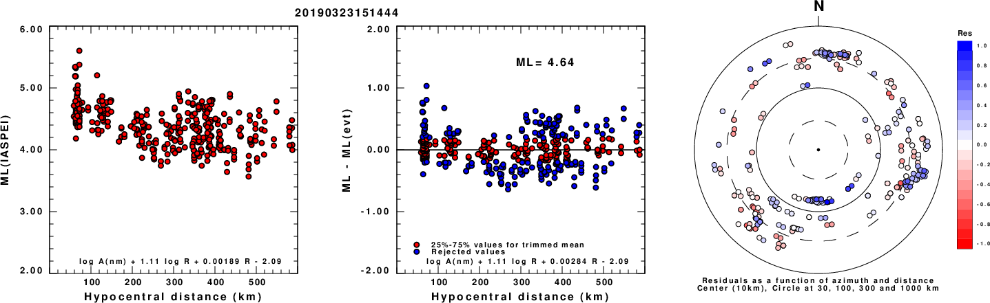
Left: ML computed using the IASPEI formula for Horizontal components. Center: ML residuals computed using a modified IASPEI formula that accounts for path specific attenuation; the values used for the trimmed mean are indicated. The ML relation used for each figure is given at the bottom of each plot.
Right: Residuals from new relation as a function of distance and azimuth.
Left: ML computed using the IASPEI formula for Vertical components (research). Center: ML residuals computed using a modified IASPEI formula that accounts for path specific attenuation; the values used for the trimmed mean are indicated. The ML relation used for each figure is given at the bottom of each plot.
Right: Residuals from new relation as a function of distance and azimuth.
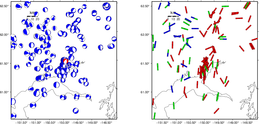
Context
The left panel of the next figure presents the focal mechanism for this earthquake (red) in the context of other nearby events (blue) in the SLU Moment Tensor Catalog. The right panel shows the inferred direction of maximum compressive stress and the type of faulting (green is strike-slip, red is normal, blue is thrust; oblique is shown by a combination of colors). Thus context plot is useful for assessing the appropriateness of the moment tensor of this event.
Waveform Inversion using wvfgrd96
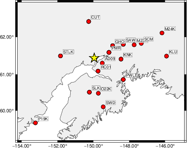
The focal mechanism was determined using broadband seismic waveforms. The location of the event (star) and the
stations used for (red) the waveform inversion are shown in the next figure.
|
|
Location of broadband stations used for waveform inversion
|
The program wvfgrd96 was used with good traces observed at short distance to determine the focal mechanism, depth and seismic moment. This technique requires a high quality signal and well determined velocity model for the Green's functions. To the extent that these are the quality data, this type of mechanism should be preferred over the radiation pattern technique which requires the separate step of defining the pressure and tension quadrants and the correct strike.
The observed and predicted traces are filtered using the following gsac commands:
cut o DIST/3.3 -40 o DIST/3.3 +50
rtr
taper w 0.1
hp c 0.03 n 3
lp c 0.08 n 3
The results of this grid search are as follow:
           DEPTH  STK   DIP  RAKE   MW    FIT
WVFGRD96    1.0    15    45    85   3.34 0.2307
WVFGRD96    2.0    15    45    85   3.49 0.3191
WVFGRD96    3.0    25    40    95   3.53 0.3069
WVFGRD96    4.0   345    70    50   3.51 0.3280
WVFGRD96    5.0   345    70    50   3.54 0.3512
WVFGRD96    6.0   345    70    45   3.55 0.3666
WVFGRD96    7.0   345    65    45   3.58 0.3753
WVFGRD96    8.0   350    60    50   3.65 0.3874
WVFGRD96    9.0   250    50    20   3.63 0.3914
WVFGRD96   10.0   255    55    30   3.65 0.4064
WVFGRD96   11.0    80    55    40   3.69 0.4196
WVFGRD96   12.0    75    60    35   3.70 0.4327
WVFGRD96   13.0   235    60   -35   3.72 0.4466
WVFGRD96   14.0   235    60   -35   3.73 0.4618
WVFGRD96   15.0   240    60   -30   3.74 0.4754
WVFGRD96   16.0   240    60   -30   3.75 0.4883
WVFGRD96   17.0   240    65   -30   3.77 0.5001
WVFGRD96   18.0   240    65   -35   3.79 0.5121
WVFGRD96   19.0   240    65   -35   3.80 0.5230
WVFGRD96   20.0   240    65   -35   3.81 0.5329
WVFGRD96   21.0   240    65   -35   3.82 0.5416
WVFGRD96   22.0   240    65   -35   3.83 0.5504
WVFGRD96   23.0   240    65   -35   3.84 0.5582
WVFGRD96   24.0   240    65   -40   3.86 0.5652
WVFGRD96   25.0   240    65   -35   3.86 0.5715
WVFGRD96   26.0   240    65   -35   3.87 0.5790
WVFGRD96   27.0   240    60   -25   3.87 0.5859
WVFGRD96   28.0   240    60   -25   3.88 0.5952
WVFGRD96   29.0   240    60   -25   3.89 0.6073
WVFGRD96   30.0   240    60   -25   3.90 0.6176
WVFGRD96   31.0   240    60   -25   3.91 0.6284
WVFGRD96   32.0   240    60   -25   3.91 0.6377
WVFGRD96   33.0   240    60   -25   3.92 0.6445
WVFGRD96   34.0   240    60   -25   3.93 0.6533
WVFGRD96   35.0   240    60   -30   3.94 0.6601
WVFGRD96   36.0   235    60   -35   3.96 0.6673
WVFGRD96   37.0   235    60   -35   3.97 0.6748
WVFGRD96   38.0   235    60   -35   3.98 0.6818
WVFGRD96   39.0   235    60   -40   4.00 0.6864
WVFGRD96   40.0   230    55   -45   4.07 0.6787
WVFGRD96   41.0   230    55   -45   4.08 0.6870
WVFGRD96   42.0   230    55   -45   4.09 0.6950
WVFGRD96   43.0   230    55   -45   4.10 0.6997
WVFGRD96   44.0   230    55   -45   4.10 0.7035
WVFGRD96   45.0   230    55   -45   4.11 0.7065
WVFGRD96   46.0   230    55   -50   4.12 0.7086
WVFGRD96   47.0   230    55   -50   4.13 0.7105
WVFGRD96   48.0   230    55   -50   4.13 0.7104
WVFGRD96   49.0   230    55   -50   4.14 0.7116
WVFGRD96   50.0   230    55   -50   4.14 0.7104
WVFGRD96   51.0   230    55   -50   4.15 0.7108
WVFGRD96   52.0   230    55   -50   4.15 0.7088
WVFGRD96   53.0   230    55   -50   4.15 0.7087
WVFGRD96   54.0   230    55   -50   4.16 0.7065
WVFGRD96   55.0   230    55   -50   4.16 0.7054
WVFGRD96   56.0   230    55   -50   4.16 0.7024
WVFGRD96   57.0   230    55   -50   4.16 0.7001
WVFGRD96   58.0   225    55   -55   4.17 0.6983
WVFGRD96   59.0   230    55   -50   4.17 0.6946
The best solution is
WVFGRD96 49.0 230 55 -50 4.14 0.7116
The mechanism corresponding to the best fit is
|
|
Figure 1. Waveform inversion focal mechanism
|
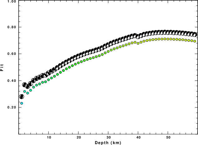
The best fit as a function of depth is given in the following figure:
|
|
Figure 2. Depth sensitivity for waveform mechanism
|
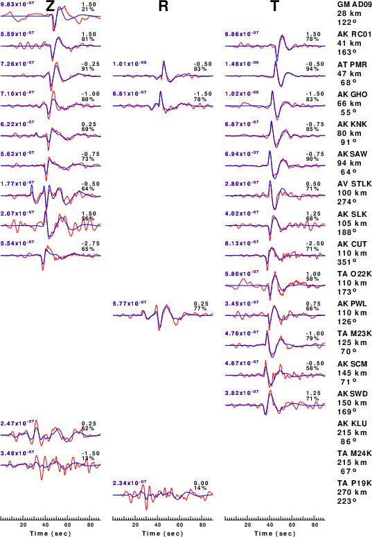
The comparison of the observed and predicted waveforms is given in the next figure. The red traces are the observed and the blue are the predicted.
Each observed-predicted component is plotted to the same scale and peak amplitudes are indicated by the numbers to the left of each trace. A pair of numbers is given in black at the right of each predicted traces. The upper number it the time shift required for maximum correlation between the observed and predicted traces. This time shift is required because the synthetics are not computed at exactly the same distance as the observed, the velocity model used in the predictions may not be perfect and the epicentral parameters may be be off.
A positive time shift indicates that the prediction is too fast and should be delayed to match the observed trace (shift to the right in this figure). A negative value indicates that the prediction is too slow. The lower number gives the percentage of variance reduction to characterize the individual goodness of fit (100% indicates a perfect fit).
The bandpass filter used in the processing and for the display was
cut o DIST/3.3 -40 o DIST/3.3 +50
rtr
taper w 0.1
hp c 0.03 n 3
lp c 0.08 n 3
|
|
Figure 3. Waveform comparison for selected depth. Red: observed; Blue - predicted. The time shift with respect to the model prediction is indicated. The percent of fit is also indicated. The time scale is relative to the first trace sample.
|
|
|
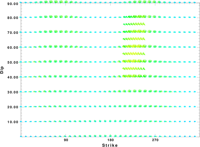
Focal mechanism sensitivity at the preferred depth. The red color indicates a very good fit to the waveforms.
Each solution is plotted as a vector at a given value of strike and dip with the angle of the vector representing the rake angle, measured, with respect to the upward vertical (N) in the figure.
|
A check on the assumed source location is possible by looking at the time shifts between the observed and predicted traces. The time shifts for waveform matching arise for several reasons:
- The origin time and epicentral distance are incorrect
- The velocity model used for the inversion is incorrect
- The velocity model used to define the P-arrival time is not the
same as the velocity model used for the waveform inversion
(assuming that the initial trace alignment is based on the
P arrival time)
Assuming only a mislocation, the time shifts are fit to a functional form:
Time_shift = A + B cos Azimuth + C Sin Azimuth
The time shifts for this inversion lead to the next figure:
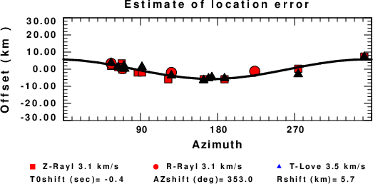
The derived shift in origin time and epicentral coordinates are given at the bottom of the figure.
Velocity Model
The WUS.model used for the waveform synthetic seismograms and for the surface wave eigenfunctions and dispersion is as follows
(The format is in the model96 format of Computer Programs in Seismology).
MODEL.01
Model after     8 iterations
ISOTROPIC
KGS
FLAT EARTH
1-D
CONSTANT VELOCITY
LINE08
LINE09
LINE10
LINE11
      H(KM)   VP(KM/S)   VS(KM/S) RHO(GM/CC)         QP         QS       ETAP       ETAS      FREFP      FREFS
     1.9000     3.4065     2.0089     2.2150  0.302E-02  0.679E-02   0.00       0.00       1.00       1.00
     6.1000     5.5445     3.2953     2.6089  0.349E-02  0.784E-02   0.00       0.00       1.00       1.00
    13.0000     6.2708     3.7396     2.7812  0.212E-02  0.476E-02   0.00       0.00       1.00       1.00
    19.0000     6.4075     3.7680     2.8223  0.111E-02  0.249E-02   0.00       0.00       1.00       1.00
     0.0000     7.9000     4.6200     3.2760  0.164E-10  0.370E-10   0.00       0.00       1.00       1.00
Last Changed Thu Apr 25 09:57:12 AM CDT 2024