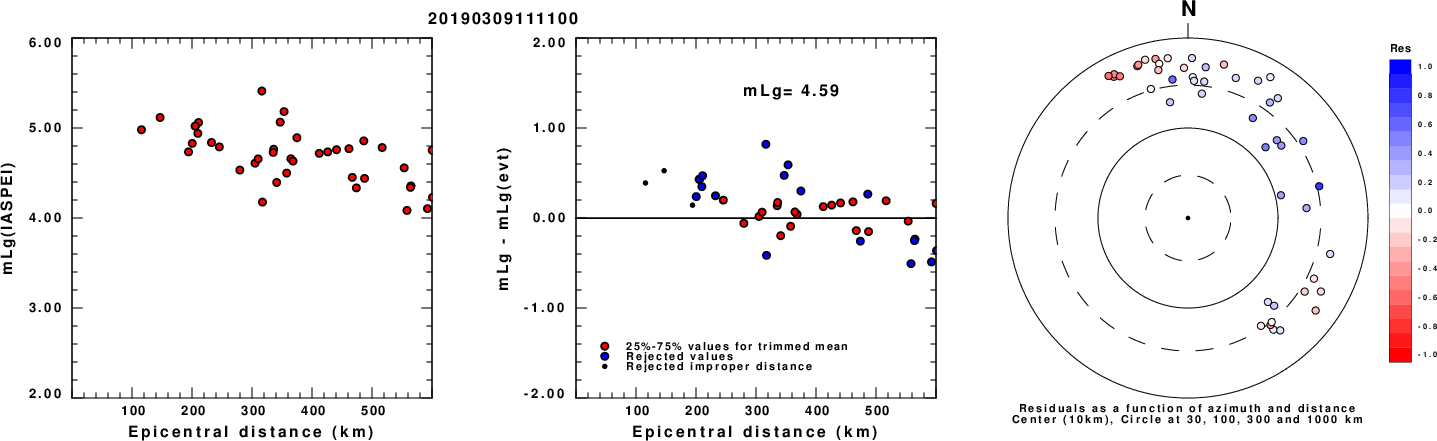
Left: mLg computed using the IASPEI formula. Center: mLg residuals versus epicentral distance ; the values used for the trimmed mean magnitude estimate are indicated. Right: residuals as a function of distance and azimuth.
The ANSS event ID is ak01934n5mur and the event page is at https://earthquake.usgs.gov/earthquakes/eventpage/ak01934n5mur/executive.
2019/03/09 11:11:00 55.276 -134.909 28.2 4.8 Alaska
 USGS/SLU Moment Tensor Solution
 ENS  2019/03/09 11:11:00:0  55.28 -134.91  28.2 4.8 Alaska

 Stations used:
   AK.BESE AK.JIS AT.CRAG AT.SIT AT.SKAG CN.BBB CN.BNAB
   CN.BUTB CN.DLBC CN.GRNB CN.HYT CN.KITB CN.MOBC CN.NDB
   CN.PCLB CN.PLBC CN.WHY CN.YUK6 TA.O30N TA.P30M TA.P32M
   TA.P33M TA.Q32M TA.R31K TA.R32K TA.R33M TA.S31K TA.S32K
   TA.S34M TA.T33K TA.T35M TA.U33K TA.U35K TA.V35K US.WRAK

 Filtering commands used:
   cut o DIST/3.3 -40 o DIST/3.3 +50
   rtr
   taper w 0.1
   hp c 0.03 n 3
   lp c 0.07 n 3

 Best Fitting Double Couple
  Mo = 1.27e+23 dyne-cm
  Mw = 4.67
  Z  = 24 km
  Plane   Strike  Dip  Rake
   NP1      295    60    40
   NP2      182    56   143
  Principal Axes:
   Axis    Value   Plunge  Azimuth
    T   1.27e+23     48     150
    N   0.00e+00     42     326
    P  -1.27e+23      2      58

 Moment Tensor: (dyne-cm)
    Component   Value
       Mxx     6.49e+21
       Mxy    -8.15e+22
       Mxz    -5.77e+22
       Myy    -7.74e+22
       Myz     2.69e+22
       Mzz     7.09e+22


                     ######--------
                 ########--------------
              ##########------------------
             ##########--------------------
           ###########----------------------
          #####----##----------------------- P
         ------------#######----------------
        ------------############----------------
        ------------###############-------------
       -------------##################-----------
       ------------#####################---------
       ------------#######################-------
       ------------#########################-----
        ------------#########################---
        ------------###########   ############--
         -----------########### T #############
          -----------##########   ############
           ----------########################
             ---------#####################
              ---------###################
                 -------###############
                     -----#########


 Global CMT Convention Moment Tensor:
      R          T          P
  7.09e+22  -5.77e+22  -2.69e+22
 -5.77e+22   6.49e+21   8.15e+22
 -2.69e+22   8.15e+22  -7.74e+22


Details of the solution is found at

http://www.eas.slu.edu/eqc/eqc_mt/MECH.NA/20190309111100/index.html
|
      STK = 295
      DIP = 60
     RAKE = 40
       MW = 4.67
       HS = 24.0
The NDK file is 20190309111100.ndk The waveform inversion is preferred.
Given the availability of digital waveforms for determination of the moment tensor, this section documents the added processing leading to mLg, if appropriate to the region, and ML by application of the respective IASPEI formulae. As a research study, the linear distance term of the IASPEI formula for ML is adjusted to remove a linear distance trend in residuals to give a regionally defined ML. The defined ML uses horizontal component recordings, but the same procedure is applied to the vertical components since there may be some interest in vertical component ground motions. Residual plots versus distance may indicate interesting features of ground motion scaling in some distance ranges. A residual plot of the regionalized magnitude is given as a function of distance and azimuth, since data sets may transcend different wave propagation provinces.
Left: mLg computed using the IASPEI formula. Center: mLg residuals versus epicentral distance ; the values used for the trimmed mean magnitude estimate are indicated.
Right: residuals as a function of distance and azimuth.
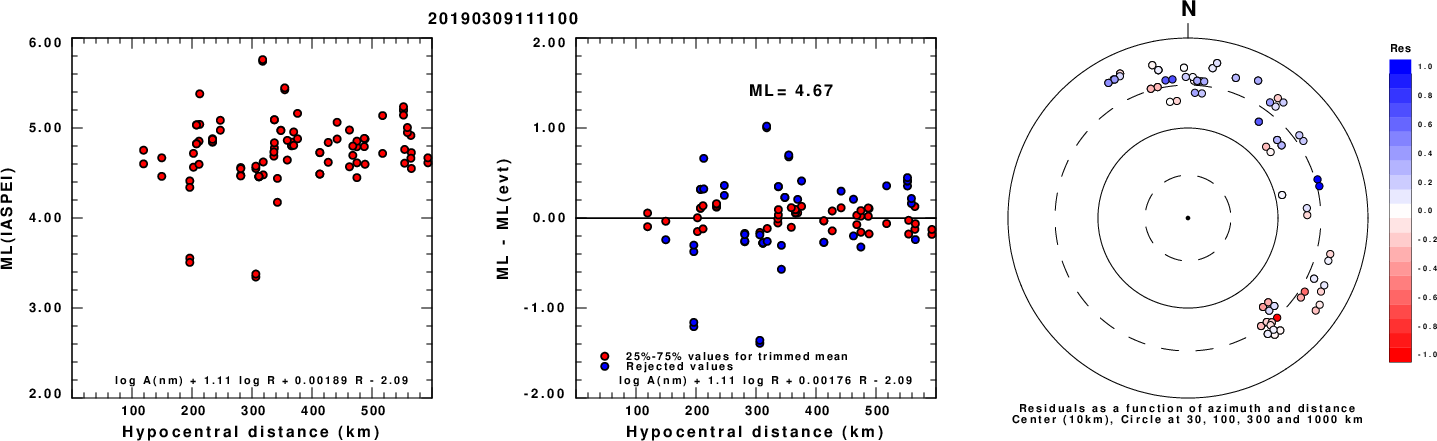
Left: ML computed using the IASPEI formula for Horizontal components. Center: ML residuals computed using a modified IASPEI formula that accounts for path specific attenuation; the values used for the trimmed mean are indicated. The ML relation used for each figure is given at the bottom of each plot.
Right: Residuals from new relation as a function of distance and azimuth.
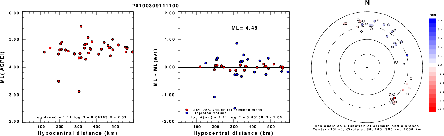
Left: ML computed using the IASPEI formula for Vertical components (research). Center: ML residuals computed using a modified IASPEI formula that accounts for path specific attenuation; the values used for the trimmed mean are indicated. The ML relation used for each figure is given at the bottom of each plot.
Right: Residuals from new relation as a function of distance and azimuth.
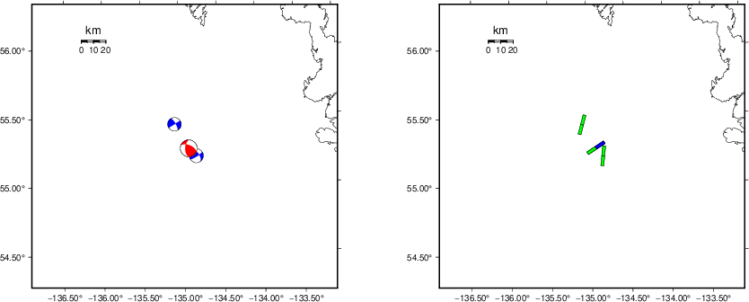 |
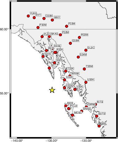
The focal mechanism was determined using broadband seismic waveforms. The location of the event (star) and the stations used for (red) the waveform inversion are shown in the next figure.
|
|
|
The program wvfgrd96 was used with good traces observed at short distance to determine the focal mechanism, depth and seismic moment. This technique requires a high quality signal and well determined velocity model for the Green's functions. To the extent that these are the quality data, this type of mechanism should be preferred over the radiation pattern technique which requires the separate step of defining the pressure and tension quadrants and the correct strike.
The observed and predicted traces are filtered using the following gsac commands:
cut o DIST/3.3 -40 o DIST/3.3 +50
rtr
taper w 0.1
hp c 0.03 n 3
lp c 0.07 n 3
The results of this grid search are as follow:
           DEPTH  STK   DIP  RAKE   MW    FIT
WVFGRD96    1.0   130    40    85   4.40 0.4745
WVFGRD96    2.0   145    45    90   4.48 0.4973
WVFGRD96    3.0   100    55   -20   4.48 0.4510
WVFGRD96    4.0   100    55   -20   4.48 0.4491
WVFGRD96    5.0   100    50   -15   4.49 0.4513
WVFGRD96    6.0   100    45   -10   4.49 0.4611
WVFGRD96    7.0   100    45   -10   4.49 0.4765
WVFGRD96    8.0   100    40    -5   4.49 0.4951
WVFGRD96    9.0   105    40    10   4.50 0.5139
WVFGRD96   10.0    90    40   -25   4.54 0.5338
WVFGRD96   11.0    90    45   -30   4.55 0.5582
WVFGRD96   12.0    90    45   -30   4.56 0.5814
WVFGRD96   13.0    90    50   -35   4.57 0.6023
WVFGRD96   14.0    90    50   -35   4.58 0.6199
WVFGRD96   15.0    90    50   -35   4.59 0.6347
WVFGRD96   16.0   300    60    50   4.58 0.6471
WVFGRD96   17.0   300    60    50   4.59 0.6612
WVFGRD96   18.0   300    60    50   4.60 0.6727
WVFGRD96   19.0   300    60    45   4.61 0.6820
WVFGRD96   20.0   300    60    50   4.64 0.6925
WVFGRD96   21.0   300    60    45   4.65 0.6988
WVFGRD96   22.0   300    60    45   4.66 0.7030
WVFGRD96   23.0   295    60    40   4.67 0.7054
WVFGRD96   24.0   295    60    40   4.67 0.7059
WVFGRD96   25.0   295    60    40   4.68 0.7045
WVFGRD96   26.0   295    60    40   4.69 0.7012
WVFGRD96   27.0   295    60    40   4.69 0.6962
WVFGRD96   28.0   295    60    40   4.70 0.6900
WVFGRD96   29.0   295    60    40   4.71 0.6823
WVFGRD96   30.0   295    60    40   4.71 0.6732
WVFGRD96   31.0   295    55    40   4.72 0.6638
WVFGRD96   32.0   295    55    35   4.73 0.6539
WVFGRD96   33.0   295    55    35   4.74 0.6428
WVFGRD96   34.0   295    55    35   4.74 0.6313
WVFGRD96   35.0   295    55    35   4.75 0.6193
WVFGRD96   36.0   295    55    35   4.76 0.6071
WVFGRD96   37.0   290    55    35   4.76 0.5950
WVFGRD96   38.0   290    55    35   4.78 0.5829
WVFGRD96   39.0   290    55    35   4.79 0.5704
WVFGRD96   40.0   295    50    35   4.86 0.5291
WVFGRD96   41.0   295    50    35   4.87 0.5180
WVFGRD96   42.0   295    50    35   4.87 0.5051
WVFGRD96   43.0   295    50    35   4.88 0.4909
WVFGRD96   44.0   290    50    35   4.88 0.4760
WVFGRD96   45.0   290    50    30   4.88 0.4610
WVFGRD96   46.0   290    50    30   4.89 0.4457
WVFGRD96   47.0   290    50    30   4.89 0.4299
WVFGRD96   48.0    70    45   -45   4.90 0.4167
WVFGRD96   49.0    70    45   -45   4.91 0.4077
WVFGRD96   50.0    70    45   -40   4.91 0.3988
The best solution is
WVFGRD96 24.0 295 60 40 4.67 0.7059
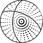
The mechanism corresponding to the best fit is
|
|
|
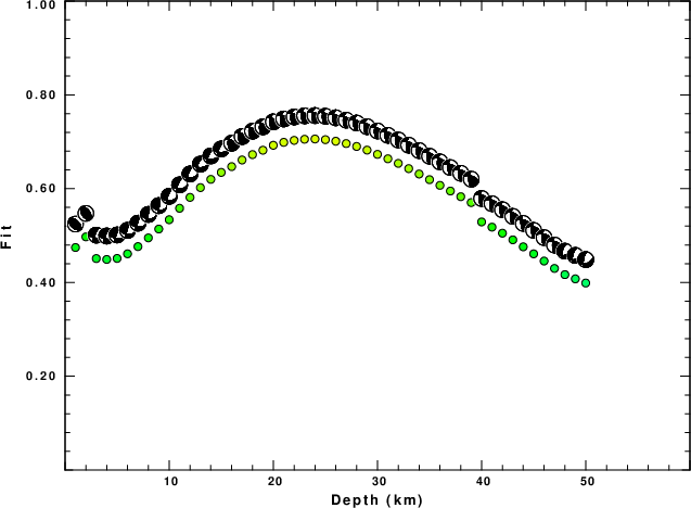
The best fit as a function of depth is given in the following figure:
|
|
|
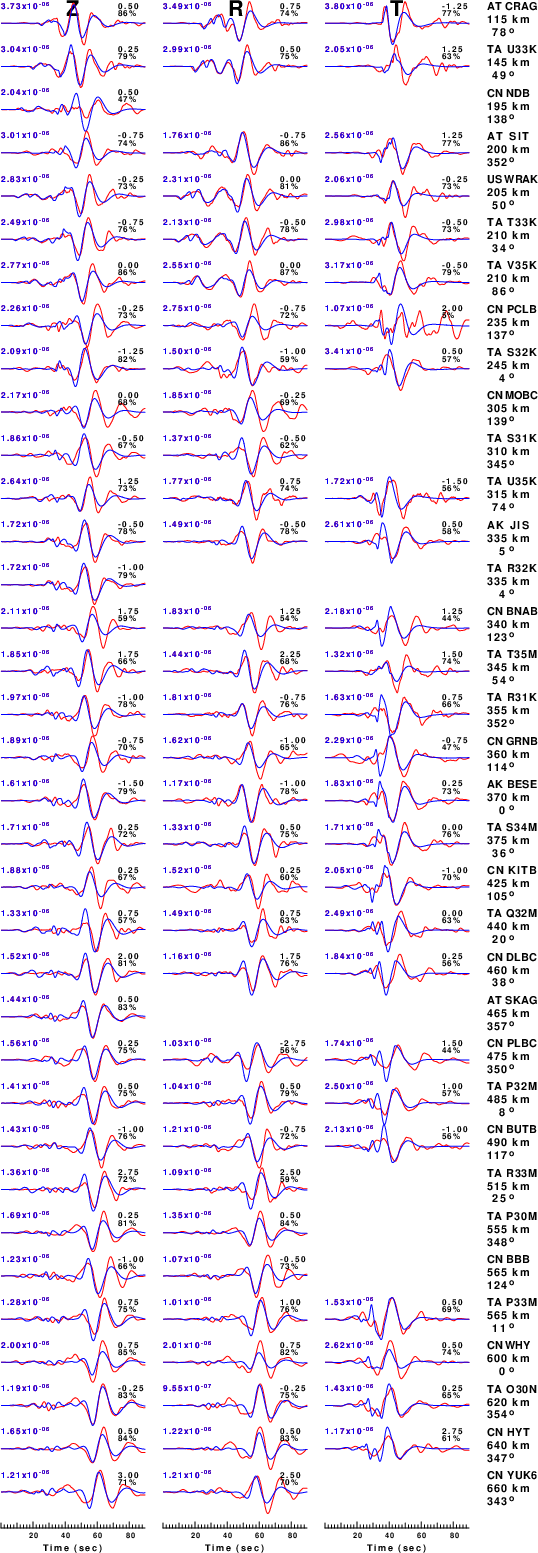
The comparison of the observed and predicted waveforms is given in the next figure. The red traces are the observed and the blue are the predicted. Each observed-predicted component is plotted to the same scale and peak amplitudes are indicated by the numbers to the left of each trace. A pair of numbers is given in black at the right of each predicted traces. The upper number it the time shift required for maximum correlation between the observed and predicted traces. This time shift is required because the synthetics are not computed at exactly the same distance as the observed, the velocity model used in the predictions may not be perfect and the epicentral parameters may be be off. A positive time shift indicates that the prediction is too fast and should be delayed to match the observed trace (shift to the right in this figure). A negative value indicates that the prediction is too slow. The lower number gives the percentage of variance reduction to characterize the individual goodness of fit (100% indicates a perfect fit).
The bandpass filter used in the processing and for the display was
cut o DIST/3.3 -40 o DIST/3.3 +50
rtr
taper w 0.1
hp c 0.03 n 3
lp c 0.07 n 3
|
| Figure 3. Waveform comparison for selected depth. Red: observed; Blue - predicted. The time shift with respect to the model prediction is indicated. The percent of fit is also indicated. The time scale is relative to the first trace sample. |
|
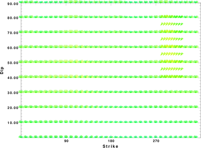
| Focal mechanism sensitivity at the preferred depth. The red color indicates a very good fit to the waveforms. Each solution is plotted as a vector at a given value of strike and dip with the angle of the vector representing the rake angle, measured, with respect to the upward vertical (N) in the figure. |
A check on the assumed source location is possible by looking at the time shifts between the observed and predicted traces. The time shifts for waveform matching arise for several reasons:
Time_shift = A + B cos Azimuth + C Sin Azimuth
The time shifts for this inversion lead to the next figure:
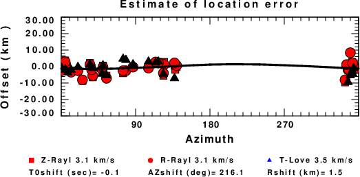
The derived shift in origin time and epicentral coordinates are given at the bottom of the figure.
The CUS.model used for the waveform synthetic seismograms and for the surface wave eigenfunctions and dispersion is as follows (The format is in the model96 format of Computer Programs in Seismology).
MODEL.01
CUS Model with Q from simple gamma values
ISOTROPIC
KGS
FLAT EARTH
1-D
CONSTANT VELOCITY
LINE08
LINE09
LINE10
LINE11
  H(KM) VP(KM/S) VS(KM/S) RHO(GM/CC)   QP   QS  ETAP  ETAS  FREFP  FREFS
  1.0000  5.0000  2.8900  2.5000 0.172E-02 0.387E-02 0.00  0.00  1.00  1.00
  9.0000  6.1000  3.5200  2.7300 0.160E-02 0.363E-02 0.00  0.00  1.00  1.00
 10.0000  6.4000  3.7000  2.8200 0.149E-02 0.336E-02 0.00  0.00  1.00  1.00
 20.0000  6.7000  3.8700  2.9020 0.000E-04 0.000E-04 0.00  0.00  1.00  1.00
  0.0000  8.1500  4.7000  3.3640 0.194E-02 0.431E-02 0.00  0.00  1.00  1.00