Location
Location ANSS
The ANSS event ID is ak01912e2f51 and the event page is at
https://earthquake.usgs.gov/earthquakes/eventpage/ak01912e2f51/executive.
2019/01/23 21:34:23 63.237 -150.573 129.1 3.9 Alaska
Focal Mechanism
 USGS/SLU Moment Tensor Solution
 ENS  2019/01/23 21:34:23:0  63.24 -150.57 129.1 3.9 Alaska

 Stations used:
   AK.BPAW AK.CAST AK.CUT AK.KTH AK.MCK AK.RND AK.SKN AK.SSN
   AK.TRF AK.WRH AT.TTA TA.H21K TA.J19K TA.J20K TA.J25K
   TA.K20K TA.M22K

 Filtering commands used:
   cut o DIST/3.4 -40 o DIST/3.4 +50
   rtr
   taper w 0.1
   hp c 0.03 n 3
   lp c 0.07 n 3

 Best Fitting Double Couple
  Mo = 2.11e+22 dyne-cm
  Mw = 4.15
  Z  = 136 km
  Plane   Strike  Dip  Rake
   NP1      204    83   -103
   NP2       85    15   -30
  Principal Axes:
   Axis    Value   Plunge  Azimuth
    T   2.11e+22     36     306
    N   0.00e+00     13     206
    P  -2.11e+22     51     100

 Moment Tensor: (dyne-cm)
    Component   Value
       Mxx     4.42e+21
       Mxy    -5.12e+21
       Mxz     7.58e+21
       Myy     8.63e+20
       Myz    -1.84e+22
       Mzz    -5.28e+21


                     ##############
                 ##################----
              ####################--------
             ####################----------
           #####################-------------
          ######   ############---------------
         ####### T ###########-----------------
        ########   ##########-------------------
        ####################--------------------
       ####################----------------------
       ###################----------   ----------
       ###################---------- P ---------#
       -#################-----------   ---------#
        ################-----------------------#
        -##############-----------------------##
         -#############----------------------##
          -###########----------------------##
           --########---------------------###
             --######-------------------###
              ----##-----------------#####
                 ---####-------########
                     ##############


 Global CMT Convention Moment Tensor:
      R          T          P
 -5.28e+21   7.58e+21   1.84e+22
  7.58e+21   4.42e+21   5.12e+21
  1.84e+22   5.12e+21   8.63e+20


Details of the solution is found at

http://www.eas.slu.edu/eqc/eqc_mt/MECH.NA/20190123213423/index.html
|
Preferred Solution
The preferred solution from an analysis of the surface-wave spectral amplitude radiation pattern, waveform inversion or first motion observations is
      STK = 85
      DIP = 15
     RAKE = -30
       MW = 4.15
       HS = 136.0
The NDK file is 20190123213423.ndk
The waveform inversion is preferred.
Magnitudes
Given the availability of digital waveforms for determination of the moment tensor, this section documents the added processing leading to mLg, if appropriate to the region, and ML by application of the respective IASPEI formulae. As a research study, the linear distance term of the IASPEI formula
for ML is adjusted to remove a linear distance trend in residuals to give a regionally defined ML. The defined ML uses horizontal component recordings, but the same procedure is applied to the vertical components since there may be some interest in vertical component ground motions. Residual plots versus distance may indicate interesting features of ground motion scaling in some distance ranges. A residual plot of the regionalized magnitude is given as a function of distance and azimuth, since data sets may transcend different wave propagation provinces.
ML Magnitude
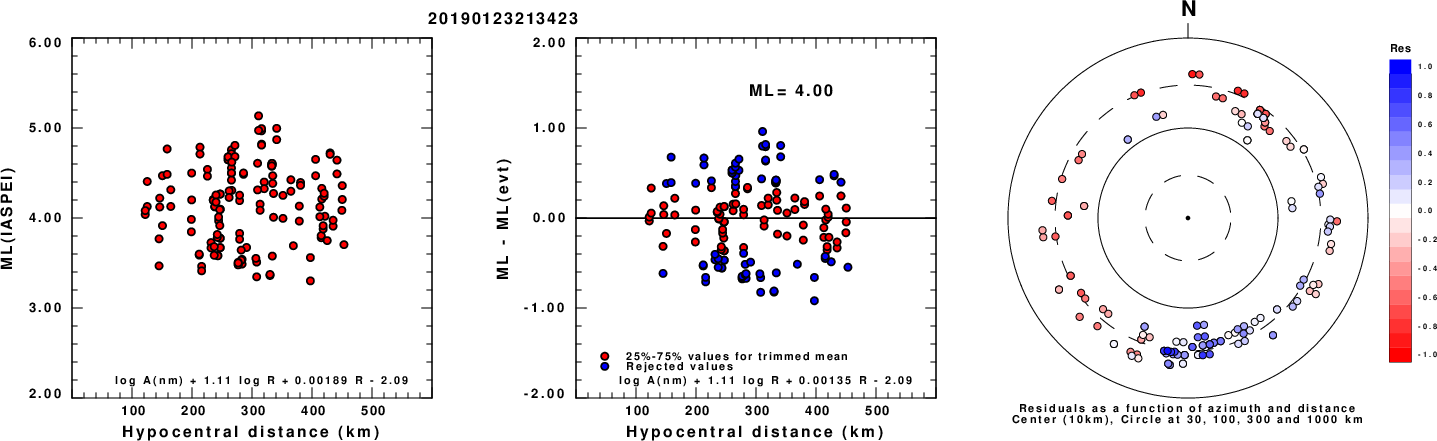
Left: ML computed using the IASPEI formula for Horizontal components. Center: ML residuals computed using a modified IASPEI formula that accounts for path specific attenuation; the values used for the trimmed mean are indicated. The ML relation used for each figure is given at the bottom of each plot.
Right: Residuals from new relation as a function of distance and azimuth.
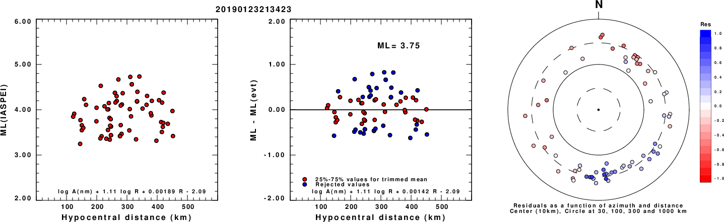
Left: ML computed using the IASPEI formula for Vertical components (research). Center: ML residuals computed using a modified IASPEI formula that accounts for path specific attenuation; the values used for the trimmed mean are indicated. The ML relation used for each figure is given at the bottom of each plot.
Right: Residuals from new relation as a function of distance and azimuth.
Context
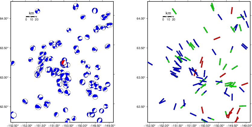
The left panel of the next figure presents the focal mechanism for this earthquake (red) in the context of other nearby events (blue) in the SLU Moment Tensor Catalog. The right panel shows the inferred direction of maximum compressive stress and the type of faulting (green is strike-slip, red is normal, blue is thrust; oblique is shown by a combination of colors). Thus context plot is useful for assessing the appropriateness of the moment tensor of this event.
Waveform Inversion using wvfgrd96
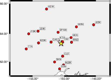
The focal mechanism was determined using broadband seismic waveforms. The location of the event (star) and the
stations used for (red) the waveform inversion are shown in the next figure.
|
|
Location of broadband stations used for waveform inversion
|
The program wvfgrd96 was used with good traces observed at short distance to determine the focal mechanism, depth and seismic moment. This technique requires a high quality signal and well determined velocity model for the Green's functions. To the extent that these are the quality data, this type of mechanism should be preferred over the radiation pattern technique which requires the separate step of defining the pressure and tension quadrants and the correct strike.
The observed and predicted traces are filtered using the following gsac commands:
cut o DIST/3.4 -40 o DIST/3.4 +50
rtr
taper w 0.1
hp c 0.03 n 3
lp c 0.07 n 3
The results of this grid search are as follow:
           DEPTH  STK   DIP  RAKE   MW    FIT
WVFGRD96    2.0    35    45    75   3.28 0.1547
WVFGRD96    4.0   185    55    30   3.28 0.1621
WVFGRD96    6.0   185    65    25   3.31 0.1820
WVFGRD96    8.0   185    70    30   3.38 0.1972
WVFGRD96   10.0   350    75   -40   3.42 0.2096
WVFGRD96   12.0   350    70   -40   3.46 0.2205
WVFGRD96   14.0   355    70   -35   3.49 0.2266
WVFGRD96   16.0    -5    70   -35   3.52 0.2283
WVFGRD96   18.0    -5    70   -30   3.54 0.2264
WVFGRD96   20.0     5    75   -25   3.57 0.2226
WVFGRD96   22.0     5    70   -25   3.59 0.2187
WVFGRD96   24.0     5    70   -20   3.61 0.2111
WVFGRD96   26.0   100    70    30   3.61 0.2012
WVFGRD96   28.0   105    70    25   3.64 0.2016
WVFGRD96   30.0   105    70    20   3.66 0.2021
WVFGRD96   32.0   105    75    15   3.68 0.2025
WVFGRD96   34.0   105    75    15   3.70 0.2023
WVFGRD96   36.0   105    80    10   3.72 0.2030
WVFGRD96   38.0   105    80    10   3.75 0.2043
WVFGRD96   40.0   105    75    20   3.79 0.2060
WVFGRD96   42.0   105    80    15   3.81 0.2083
WVFGRD96   44.0   105    85    10   3.83 0.2123
WVFGRD96   46.0   285    90    -5   3.85 0.2173
WVFGRD96   48.0   285    80    10   3.86 0.2267
WVFGRD96   50.0   285    80    10   3.88 0.2372
WVFGRD96   52.0   285    80    10   3.90 0.2470
WVFGRD96   54.0   285    80    15   3.91 0.2564
WVFGRD96   56.0   285    80    15   3.93 0.2647
WVFGRD96   58.0   285    80    15   3.94 0.2707
WVFGRD96   60.0   285    80    15   3.95 0.2762
WVFGRD96   62.0   285    80    15   3.96 0.2817
WVFGRD96   64.0   285    80    15   3.97 0.2877
WVFGRD96   66.0   285    80    15   3.98 0.2941
WVFGRD96   68.0   285    80    15   3.99 0.3044
WVFGRD96   70.0   285    85    15   4.01 0.3141
WVFGRD96   72.0   285    85    15   4.02 0.3245
WVFGRD96   74.0   105    85   -10   4.03 0.3332
WVFGRD96   76.0   100    80   -15   4.02 0.3445
WVFGRD96   78.0   100    65   -10   4.02 0.3547
WVFGRD96   80.0   120    35    10   4.03 0.3787
WVFGRD96   82.0   115    30     5   4.04 0.4174
WVFGRD96   84.0   115    30     5   4.06 0.4536
WVFGRD96   86.0   115    25     5   4.07 0.4840
WVFGRD96   88.0   115    25     5   4.08 0.5073
WVFGRD96   90.0   110    20     0   4.08 0.5195
WVFGRD96   92.0   110    20     0   4.09 0.5309
WVFGRD96   94.0   110    20     0   4.09 0.5402
WVFGRD96   96.0   110    20     0   4.10 0.5482
WVFGRD96   98.0   105    15    -5   4.10 0.5576
WVFGRD96  100.0   105    15    -5   4.11 0.5651
WVFGRD96  102.0   100    15   -10   4.11 0.5727
WVFGRD96  104.0   100    15   -10   4.11 0.5802
WVFGRD96  106.0   100    15   -10   4.12 0.5865
WVFGRD96  108.0    85    15   -25   4.12 0.5927
WVFGRD96  110.0    70    10   -40   4.12 0.6005
WVFGRD96  112.0    70    10   -40   4.13 0.6083
WVFGRD96  114.0    75    10   -35   4.13 0.6144
WVFGRD96  116.0    75    10   -35   4.13 0.6193
WVFGRD96  118.0    75    10   -35   4.13 0.6245
WVFGRD96  120.0    75    10   -35   4.14 0.6289
WVFGRD96  122.0    75    10   -35   4.14 0.6324
WVFGRD96  124.0    75    10   -35   4.14 0.6365
WVFGRD96  126.0    75    10   -35   4.14 0.6380
WVFGRD96  128.0    85    15   -25   4.14 0.6399
WVFGRD96  130.0    85    15   -25   4.14 0.6428
WVFGRD96  132.0    85    15   -25   4.14 0.6436
WVFGRD96  134.0    85    15   -30   4.15 0.6432
WVFGRD96  136.0    85    15   -30   4.15 0.6454
WVFGRD96  138.0    85    15   -25   4.15 0.6453
WVFGRD96  140.0    85    15   -30   4.15 0.6440
WVFGRD96  142.0    85    15   -30   4.15 0.6448
WVFGRD96  144.0    85    15   -30   4.15 0.6444
WVFGRD96  146.0    85    15   -30   4.15 0.6423
WVFGRD96  148.0    85    15   -30   4.16 0.6419
WVFGRD96  150.0    85    15   -30   4.16 0.6403
WVFGRD96  152.0    85    15   -30   4.16 0.6380
WVFGRD96  154.0    85    15   -30   4.16 0.6366
WVFGRD96  156.0    85    15   -30   4.16 0.6353
WVFGRD96  158.0    85    15   -30   4.16 0.6327
The best solution is
WVFGRD96 136.0 85 15 -30 4.15 0.6454
The mechanism corresponding to the best fit is
|
|
Figure 1. Waveform inversion focal mechanism
|
The best fit as a function of depth is given in the following figure:
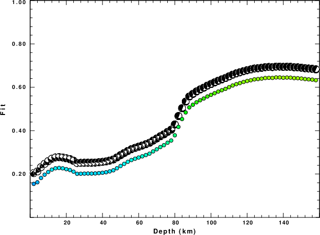
|
|
Figure 2. Depth sensitivity for waveform mechanism
|
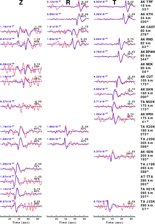
The comparison of the observed and predicted waveforms is given in the next figure. The red traces are the observed and the blue are the predicted.
Each observed-predicted component is plotted to the same scale and peak amplitudes are indicated by the numbers to the left of each trace. A pair of numbers is given in black at the right of each predicted traces. The upper number it the time shift required for maximum correlation between the observed and predicted traces. This time shift is required because the synthetics are not computed at exactly the same distance as the observed, the velocity model used in the predictions may not be perfect and the epicentral parameters may be be off.
A positive time shift indicates that the prediction is too fast and should be delayed to match the observed trace (shift to the right in this figure). A negative value indicates that the prediction is too slow. The lower number gives the percentage of variance reduction to characterize the individual goodness of fit (100% indicates a perfect fit).
The bandpass filter used in the processing and for the display was
cut o DIST/3.4 -40 o DIST/3.4 +50
rtr
taper w 0.1
hp c 0.03 n 3
lp c 0.07 n 3
|
|
Figure 3. Waveform comparison for selected depth. Red: observed; Blue - predicted. The time shift with respect to the model prediction is indicated. The percent of fit is also indicated. The time scale is relative to the first trace sample.
|
|
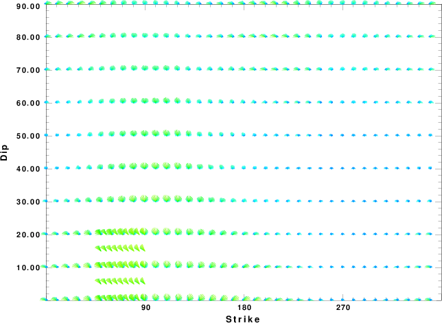
|
Focal mechanism sensitivity at the preferred depth. The red color indicates a very good fit to the waveforms.
Each solution is plotted as a vector at a given value of strike and dip with the angle of the vector representing the rake angle, measured, with respect to the upward vertical (N) in the figure.
|
A check on the assumed source location is possible by looking at the time shifts between the observed and predicted traces. The time shifts for waveform matching arise for several reasons:
- The origin time and epicentral distance are incorrect
- The velocity model used for the inversion is incorrect
- The velocity model used to define the P-arrival time is not the
same as the velocity model used for the waveform inversion
(assuming that the initial trace alignment is based on the
P arrival time)
Assuming only a mislocation, the time shifts are fit to a functional form:
Time_shift = A + B cos Azimuth + C Sin Azimuth
The time shifts for this inversion lead to the next figure:
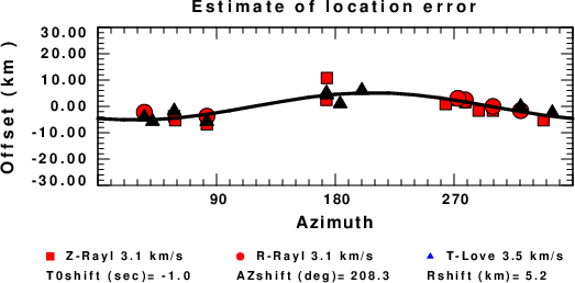
The derived shift in origin time and epicentral coordinates are given at the bottom of the figure.
Velocity Model
The WUS.model used for the waveform synthetic seismograms and for the surface wave eigenfunctions and dispersion is as follows
(The format is in the model96 format of Computer Programs in Seismology).
MODEL.01
Model after     8 iterations
ISOTROPIC
KGS
FLAT EARTH
1-D
CONSTANT VELOCITY
LINE08
LINE09
LINE10
LINE11
      H(KM)   VP(KM/S)   VS(KM/S) RHO(GM/CC)         QP         QS       ETAP       ETAS      FREFP      FREFS
     1.9000     3.4065     2.0089     2.2150  0.302E-02  0.679E-02   0.00       0.00       1.00       1.00
     6.1000     5.5445     3.2953     2.6089  0.349E-02  0.784E-02   0.00       0.00       1.00       1.00
    13.0000     6.2708     3.7396     2.7812  0.212E-02  0.476E-02   0.00       0.00       1.00       1.00
    19.0000     6.4075     3.7680     2.8223  0.111E-02  0.249E-02   0.00       0.00       1.00       1.00
     0.0000     7.9000     4.6200     3.2760  0.164E-10  0.370E-10   0.00       0.00       1.00       1.00
Last Changed Thu Apr 25 08:25:28 AM CDT 2024