Location
Location ANSS
The ANSS event ID is ak018gl9gvsc and the event page is at
https://earthquake.usgs.gov/earthquakes/eventpage/ak018gl9gvsc/executive.
2018/12/27 14:21:13 61.286 -150.068 41.0 4.8 Alaska
Focal Mechanism
 USGS/SLU Moment Tensor Solution
 ENS  2018/12/27 14:21:13:0  61.29 -150.07  41.0 4.8 Alaska

 Stations used:
   AK.BRLK AK.CAST AK.CNP AK.DHY AK.FID AK.GHO AK.GLB AK.GLI
   AK.HOM AK.KNK AK.KTH AK.PWL AK.RND AK.SAW AK.SCM AK.SKN
   AK.SSN AK.SWD AK.VRDI AT.PMR AV.ILSW AV.SPU AV.STLK GM.AD09
   GM.AD11 TA.M20K TA.O22K TA.P19K

 Filtering commands used:
   cut o DIST/3.3 -40 o DIST/3.3 +50
   rtr
   taper w 0.1
   hp c 0.03 n 3
   lp c 0.10 n 3

 Best Fitting Double Couple
  Mo = 1.46e+23 dyne-cm
  Mw = 4.71
  Z  = 47 km
  Plane   Strike  Dip  Rake
   NP1      185    75   -65
   NP2      304    29   -148
  Principal Axes:
   Axis    Value   Plunge  Azimuth
    T   1.46e+23     26     256
    N   0.00e+00     24     358
    P  -1.46e+23     53     125

 Moment Tensor: (dyne-cm)
    Component   Value
       Mxx    -9.86e+21
       Mxy     5.30e+22
       Mxz     2.59e+22
       Myy     7.61e+22
       Myz    -1.13e+23
       Mzz    -6.63e+22


                     --------######
                 -----------###########
              -----########--#############
             -#############-------#########
           ###############-----------########
          ################-------------#######
         ################----------------######
        #################-----------------######
        #################-------------------####
       #################--------------------#####
       #################---------------------####
       #################----------------------###
       ####   ##########----------   ---------###
        ### T ##########---------- P ---------##
        ###   ##########----------   ---------##
         ###############----------------------#
          ##############----------------------
           #############---------------------
             ###########-------------------
              ###########-----------------
                 ########--------------
                     #####---------


 Global CMT Convention Moment Tensor:
      R          T          P
 -6.63e+22   2.59e+22   1.13e+23
  2.59e+22  -9.86e+21  -5.30e+22
  1.13e+23  -5.30e+22   7.61e+22


Details of the solution is found at

http://www.eas.slu.edu/eqc/eqc_mt/MECH.NA/20181227142113/index.html
|
Preferred Solution
The preferred solution from an analysis of the surface-wave spectral amplitude radiation pattern, waveform inversion or first motion observations is
      STK = 185
      DIP = 75
     RAKE = -65
       MW = 4.71
       HS = 47.0
The NDK file is 20181227142113.ndk
The waveform inversion is preferred.
Moment Tensor Comparison
The following compares this source inversion to those provided by others. The purpose is to look for major differences and also to note slight differences that might be inherent to the processing procedure. For completeness the USGS/SLU solution is repeated from above.
| SLU |
USGSMWR |
USGSW |
 USGS/SLU Moment Tensor Solution
 ENS  2018/12/27 14:21:13:0  61.29 -150.07  41.0 4.8 Alaska

 Stations used:
   AK.BRLK AK.CAST AK.CNP AK.DHY AK.FID AK.GHO AK.GLB AK.GLI
   AK.HOM AK.KNK AK.KTH AK.PWL AK.RND AK.SAW AK.SCM AK.SKN
   AK.SSN AK.SWD AK.VRDI AT.PMR AV.ILSW AV.SPU AV.STLK GM.AD09
   GM.AD11 TA.M20K TA.O22K TA.P19K

 Filtering commands used:
   cut o DIST/3.3 -40 o DIST/3.3 +50
   rtr
   taper w 0.1
   hp c 0.03 n 3
   lp c 0.10 n 3

 Best Fitting Double Couple
  Mo = 1.46e+23 dyne-cm
  Mw = 4.71
  Z  = 47 km
  Plane   Strike  Dip  Rake
   NP1      185    75   -65
   NP2      304    29   -148
  Principal Axes:
   Axis    Value   Plunge  Azimuth
    T   1.46e+23     26     256
    N   0.00e+00     24     358
    P  -1.46e+23     53     125

 Moment Tensor: (dyne-cm)
    Component   Value
       Mxx    -9.86e+21
       Mxy     5.30e+22
       Mxz     2.59e+22
       Myy     7.61e+22
       Myz    -1.13e+23
       Mzz    -6.63e+22


                     --------######
                 -----------###########
              -----########--#############
             -#############-------#########
           ###############-----------########
          ################-------------#######
         ################----------------######
        #################-----------------######
        #################-------------------####
       #################--------------------#####
       #################---------------------####
       #################----------------------###
       ####   ##########----------   ---------###
        ### T ##########---------- P ---------##
        ###   ##########----------   ---------##
         ###############----------------------#
          ##############----------------------
           #############---------------------
             ###########-------------------
              ###########-----------------
                 ########--------------
                     #####---------


 Global CMT Convention Moment Tensor:
      R          T          P
 -6.63e+22   2.59e+22   1.13e+23
  2.59e+22  -9.86e+21  -5.30e+22
  1.13e+23  -5.30e+22   7.61e+22


Details of the solution is found at

http://www.eas.slu.edu/eqc/eqc_mt/MECH.NA/20181227142113/index.html
|
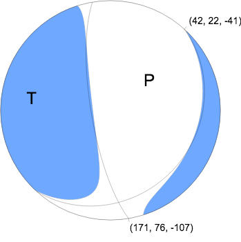
Regional Moment Tensor (Mwr)
Moment 2.017e+16 N-m
Magnitude 4.80 Mwr
Depth 54.0 km
Percent DC 79%
Half Duration -
Catalog US
Data Source US 3
Contributor US 3
Nodal Planes
Plane Strike Dip Rake
NP1 171 76 -107
NP2 42 22 -41
Principal Axes
Axis Value Plunge Azimuth
T 2.118e+16 N-m 29 274
N -0.218e+16 N-m 17 175
P -1.899e+16 N-m 56 58
|
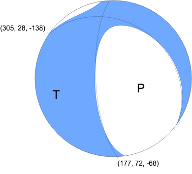
W-phase Moment Tensor (Mww) Preferred
Moment 2.107e+16 N-m
Magnitude 4.82 Mww
Depth 45.5 km
Percent DC 84%
Half Duration 0.66 s
Catalog US
Data Source US 3
Contributor US 3
Nodal Planes
Plane Strike Dip Rake
NP1 305 28 -138
NP2 177 72 -68
Principal Axes
Axis Value Plunge Azimuth
T 2.015e+16 N-m 24 250
N 0.174e+16 N-m 21 350
P -2.189e+16 N-m 58 117
|
Magnitudes
Given the availability of digital waveforms for determination of the moment tensor, this section documents the added processing leading to mLg, if appropriate to the region, and ML by application of the respective IASPEI formulae. As a research study, the linear distance term of the IASPEI formula
for ML is adjusted to remove a linear distance trend in residuals to give a regionally defined ML. The defined ML uses horizontal component recordings, but the same procedure is applied to the vertical components since there may be some interest in vertical component ground motions. Residual plots versus distance may indicate interesting features of ground motion scaling in some distance ranges. A residual plot of the regionalized magnitude is given as a function of distance and azimuth, since data sets may transcend different wave propagation provinces.
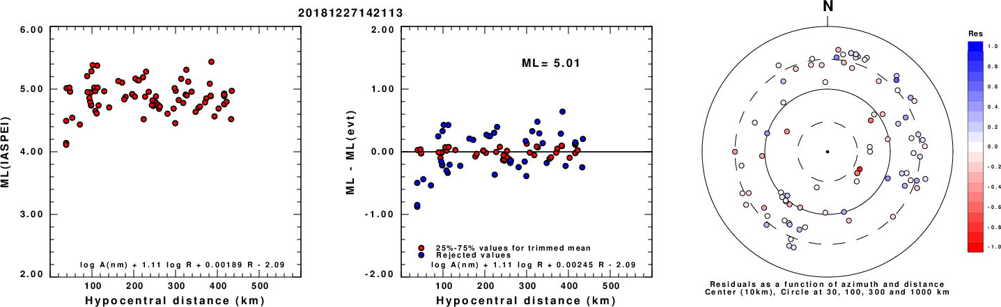
ML Magnitude
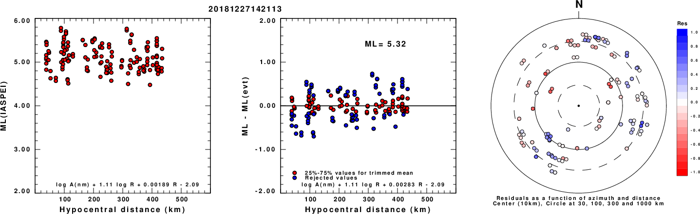
Left: ML computed using the IASPEI formula for Horizontal components. Center: ML residuals computed using a modified IASPEI formula that accounts for path specific attenuation; the values used for the trimmed mean are indicated. The ML relation used for each figure is given at the bottom of each plot.
Right: Residuals from new relation as a function of distance and azimuth.
Left: ML computed using the IASPEI formula for Vertical components (research). Center: ML residuals computed using a modified IASPEI formula that accounts for path specific attenuation; the values used for the trimmed mean are indicated. The ML relation used for each figure is given at the bottom of each plot.
Right: Residuals from new relation as a function of distance and azimuth.
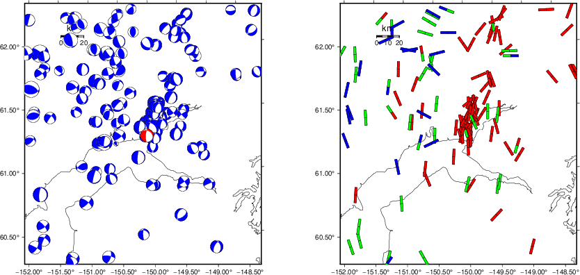
Context
The left panel of the next figure presents the focal mechanism for this earthquake (red) in the context of other nearby events (blue) in the SLU Moment Tensor Catalog. The right panel shows the inferred direction of maximum compressive stress and the type of faulting (green is strike-slip, red is normal, blue is thrust; oblique is shown by a combination of colors). Thus context plot is useful for assessing the appropriateness of the moment tensor of this event.
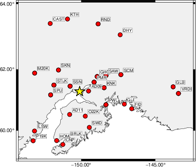
Waveform Inversion using wvfgrd96
The focal mechanism was determined using broadband seismic waveforms. The location of the event (star) and the
stations used for (red) the waveform inversion are shown in the next figure.
|
|
Location of broadband stations used for waveform inversion
|
The program wvfgrd96 was used with good traces observed at short distance to determine the focal mechanism, depth and seismic moment. This technique requires a high quality signal and well determined velocity model for the Green's functions. To the extent that these are the quality data, this type of mechanism should be preferred over the radiation pattern technique which requires the separate step of defining the pressure and tension quadrants and the correct strike.
The observed and predicted traces are filtered using the following gsac commands:
cut o DIST/3.3 -40 o DIST/3.3 +50
rtr
taper w 0.1
hp c 0.03 n 3
lp c 0.10 n 3
The results of this grid search are as follow:
           DEPTH  STK   DIP  RAKE   MW    FIT
WVFGRD96    1.0   180    45    85   3.75 0.1283
WVFGRD96    2.0   185    45    90   3.92 0.1803
WVFGRD96    3.0   165    45    60   3.96 0.1614
WVFGRD96    4.0   155    45    35   3.96 0.1582
WVFGRD96    5.0   290    30   -10   3.97 0.1772
WVFGRD96    6.0   350    90    45   4.00 0.2027
WVFGRD96    7.0   150    80   -40   4.04 0.2258
WVFGRD96    8.0   155    85   -45   4.10 0.2428
WVFGRD96    9.0   155    85   -45   4.12 0.2604
WVFGRD96   10.0   165    80   -40   4.15 0.2769
WVFGRD96   11.0   165    80   -40   4.17 0.2920
WVFGRD96   12.0   240    60    40   4.21 0.3050
WVFGRD96   13.0     0    75    45   4.21 0.3193
WVFGRD96   14.0     0    75    45   4.22 0.3312
WVFGRD96   15.0     0    75    45   4.24 0.3419
WVFGRD96   16.0     0    75    45   4.26 0.3511
WVFGRD96   17.0     0    75    45   4.28 0.3590
WVFGRD96   18.0     0    80    45   4.29 0.3670
WVFGRD96   19.0    35    70    50   4.32 0.3745
WVFGRD96   20.0    35    70    50   4.34 0.3839
WVFGRD96   21.0    35    70    55   4.36 0.3941
WVFGRD96   22.0    35    70    55   4.38 0.4052
WVFGRD96   23.0    35    70    55   4.40 0.4157
WVFGRD96   24.0    25    80    55   4.40 0.4285
WVFGRD96   25.0    25    80    55   4.41 0.4422
WVFGRD96   26.0    20    85    50   4.42 0.4570
WVFGRD96   27.0    20    85    50   4.44 0.4716
WVFGRD96   28.0    20    85    55   4.45 0.4846
WVFGRD96   29.0    20    85    55   4.47 0.4967
WVFGRD96   30.0    25    85    55   4.48 0.5106
WVFGRD96   31.0    20    90    55   4.49 0.5248
WVFGRD96   32.0    20    90    60   4.50 0.5407
WVFGRD96   33.0    20    90    60   4.51 0.5543
WVFGRD96   34.0    20    90    60   4.52 0.5664
WVFGRD96   35.0   195    85   -60   4.52 0.5805
WVFGRD96   36.0   195    85   -60   4.53 0.5902
WVFGRD96   37.0   195    85   -60   4.54 0.5986
WVFGRD96   38.0   195    85   -60   4.54 0.6044
WVFGRD96   39.0   190    80   -55   4.55 0.6088
WVFGRD96   40.0   195    85   -65   4.67 0.6073
WVFGRD96   41.0   190    80   -65   4.67 0.6130
WVFGRD96   42.0   190    80   -65   4.68 0.6190
WVFGRD96   43.0   190    80   -65   4.68 0.6247
WVFGRD96   44.0   190    80   -65   4.69 0.6288
WVFGRD96   45.0   190    80   -65   4.70 0.6317
WVFGRD96   46.0   185    75   -65   4.70 0.6335
WVFGRD96   47.0   185    75   -65   4.71 0.6346
WVFGRD96   48.0   185    75   -65   4.72 0.6336
WVFGRD96   49.0   185    75   -65   4.72 0.6324
WVFGRD96   50.0   185    75   -65   4.73 0.6298
WVFGRD96   51.0   185    75   -65   4.73 0.6264
WVFGRD96   52.0   185    75   -65   4.74 0.6218
WVFGRD96   53.0   185    75   -65   4.74 0.6160
WVFGRD96   54.0   185    75   -65   4.74 0.6094
WVFGRD96   55.0   185    75   -65   4.75 0.6016
WVFGRD96   56.0   190    80   -65   4.75 0.5942
WVFGRD96   57.0   185    80   -65   4.76 0.5861
WVFGRD96   58.0   185    80   -65   4.76 0.5790
WVFGRD96   59.0   185    80   -65   4.76 0.5716
The best solution is
WVFGRD96 47.0 185 75 -65 4.71 0.6346
The mechanism corresponding to the best fit is
|
|
Figure 1. Waveform inversion focal mechanism
|
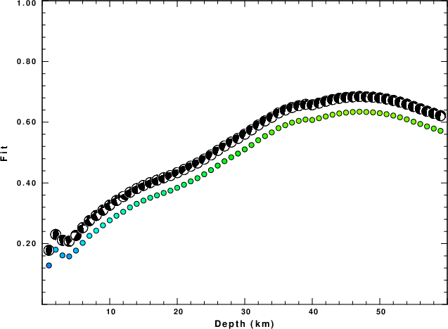
The best fit as a function of depth is given in the following figure:
|
|
Figure 2. Depth sensitivity for waveform mechanism
|
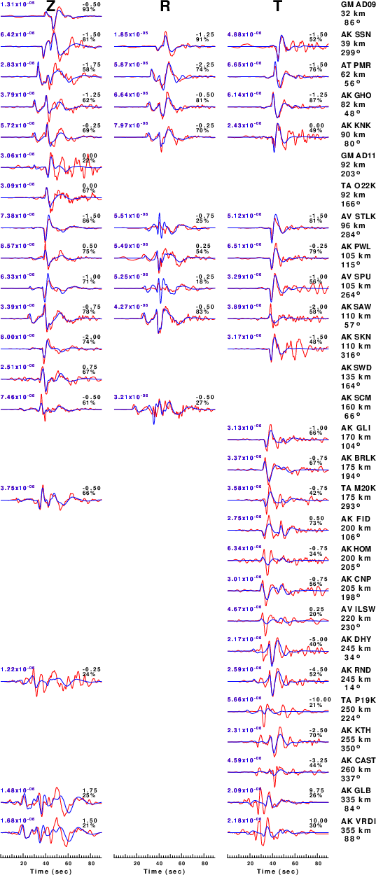
The comparison of the observed and predicted waveforms is given in the next figure. The red traces are the observed and the blue are the predicted.
Each observed-predicted component is plotted to the same scale and peak amplitudes are indicated by the numbers to the left of each trace. A pair of numbers is given in black at the right of each predicted traces. The upper number it the time shift required for maximum correlation between the observed and predicted traces. This time shift is required because the synthetics are not computed at exactly the same distance as the observed, the velocity model used in the predictions may not be perfect and the epicentral parameters may be be off.
A positive time shift indicates that the prediction is too fast and should be delayed to match the observed trace (shift to the right in this figure). A negative value indicates that the prediction is too slow. The lower number gives the percentage of variance reduction to characterize the individual goodness of fit (100% indicates a perfect fit).
The bandpass filter used in the processing and for the display was
cut o DIST/3.3 -40 o DIST/3.3 +50
rtr
taper w 0.1
hp c 0.03 n 3
lp c 0.10 n 3
|
|
Figure 3. Waveform comparison for selected depth. Red: observed; Blue - predicted. The time shift with respect to the model prediction is indicated. The percent of fit is also indicated. The time scale is relative to the first trace sample.
|
|
|
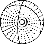
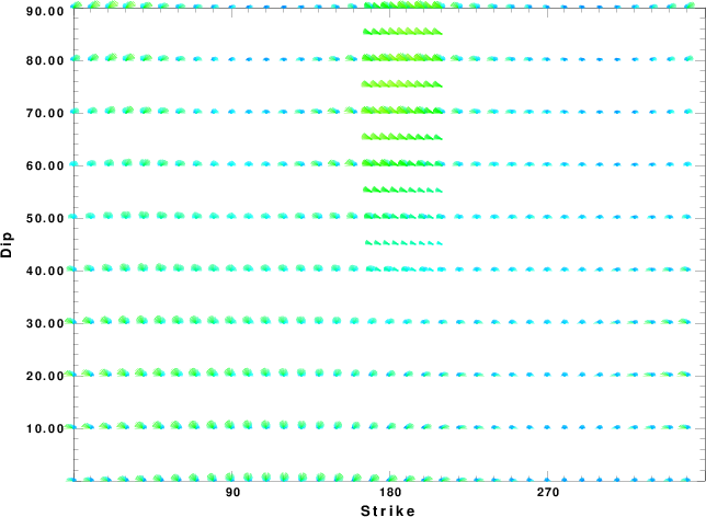
Focal mechanism sensitivity at the preferred depth. The red color indicates a very good fit to the waveforms.
Each solution is plotted as a vector at a given value of strike and dip with the angle of the vector representing the rake angle, measured, with respect to the upward vertical (N) in the figure.
|
A check on the assumed source location is possible by looking at the time shifts between the observed and predicted traces. The time shifts for waveform matching arise for several reasons:
- The origin time and epicentral distance are incorrect
- The velocity model used for the inversion is incorrect
- The velocity model used to define the P-arrival time is not the
same as the velocity model used for the waveform inversion
(assuming that the initial trace alignment is based on the
P arrival time)
Assuming only a mislocation, the time shifts are fit to a functional form:
Time_shift = A + B cos Azimuth + C Sin Azimuth
The time shifts for this inversion lead to the next figure:
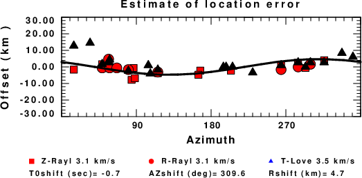
The derived shift in origin time and epicentral coordinates are given at the bottom of the figure.
Velocity Model
The WUS.model used for the waveform synthetic seismograms and for the surface wave eigenfunctions and dispersion is as follows
(The format is in the model96 format of Computer Programs in Seismology).
MODEL.01
Model after     8 iterations
ISOTROPIC
KGS
FLAT EARTH
1-D
CONSTANT VELOCITY
LINE08
LINE09
LINE10
LINE11
      H(KM)   VP(KM/S)   VS(KM/S) RHO(GM/CC)         QP         QS       ETAP       ETAS      FREFP      FREFS
     1.9000     3.4065     2.0089     2.2150  0.302E-02  0.679E-02   0.00       0.00       1.00       1.00
     6.1000     5.5445     3.2953     2.6089  0.349E-02  0.784E-02   0.00       0.00       1.00       1.00
    13.0000     6.2708     3.7396     2.7812  0.212E-02  0.476E-02   0.00       0.00       1.00       1.00
    19.0000     6.4075     3.7680     2.8223  0.111E-02  0.249E-02   0.00       0.00       1.00       1.00
     0.0000     7.9000     4.6200     3.2760  0.164E-10  0.370E-10   0.00       0.00       1.00       1.00
Last Changed Fri Apr 26 05:17:23 AM CDT 2024