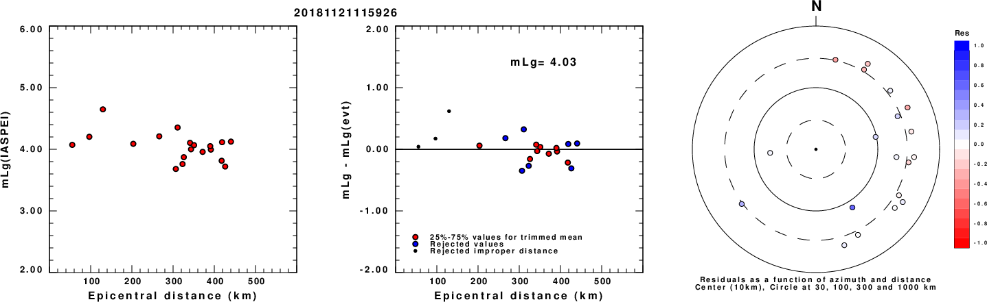
Left: mLg computed using the IASPEI formula. Center: mLg residuals versus epicentral distance ; the values used for the trimmed mean magnitude estimate are indicated. Right: residuals as a function of distance and azimuth.
The ANSS event ID is ak018exok9gi and the event page is at https://earthquake.usgs.gov/earthquakes/eventpage/ak018exok9gi/executive.
2018/11/21 11:59:26 65.573 -166.783 10.8 4 Alaska
 USGS/SLU Moment Tensor Solution
 ENS  2018/11/21 11:59:26:0  65.57 -166.78  10.8 4.0 Alaska

 Stations used:
   AK.ANM AK.GAMB AK.RDOG AK.TNA TA.C18K TA.E18K TA.F15K
   TA.F17K TA.F19K TA.G16K TA.G18K TA.H17K TA.H18K TA.I17K
   TA.J14K TA.J16K TA.J17K

 Filtering commands used:
   cut o DIST/3.3 -40 o DIST/3.3 +50
   rtr
   taper w 0.1
   hp c 0.03 n 3
   lp c 0.10 n 3

 Best Fitting Double Couple
  Mo = 7.24e+21 dyne-cm
  Mw = 3.84
  Z  = 15 km
  Plane   Strike  Dip  Rake
   NP1       73    57   -130
   NP2      310    50   -45
  Principal Axes:
   Axis    Value   Plunge  Azimuth
    T   7.24e+21      4     190
    N   0.00e+00     33      97
    P  -7.24e+21     57     286

 Moment Tensor: (dyne-cm)
    Component   Value
       Mxx     6.82e+21
       Mxy     1.80e+21
       Mxz    -1.44e+21
       Myy    -1.78e+21
       Myz     3.09e+21
       Mzz    -5.04e+21


                     ##############
                 ######################
              ############################
             #--------#####################
           -----------------#################
          ---------------------###############
         -------------------------#############
        ----------------------------############
        ----------   -----------------#########-
       ----------- P ------------------#######---
       -----------   -------------------#####----
       -----------------------------------#------
       ----------------------------------#-------
        ------------------------------#####-----
        #-------------------------##########----
         ####----------------###############---
          ##################################--
           #################################-
             ##############################
              ############################
                 ######   #############
                     ## T #########


 Global CMT Convention Moment Tensor:
      R          T          P
 -5.04e+21  -1.44e+21  -3.09e+21
 -1.44e+21   6.82e+21  -1.80e+21
 -3.09e+21  -1.80e+21  -1.78e+21


Details of the solution is found at

http://www.eas.slu.edu/eqc/eqc_mt/MECH.NA/20181121115926/index.html
|
      STK = 310
      DIP = 50
     RAKE = -45
       MW = 3.84
       HS = 15.0
The NDK file is 20181121115926.ndk The waveform inversion is preferred.
Given the availability of digital waveforms for determination of the moment tensor, this section documents the added processing leading to mLg, if appropriate to the region, and ML by application of the respective IASPEI formulae. As a research study, the linear distance term of the IASPEI formula for ML is adjusted to remove a linear distance trend in residuals to give a regionally defined ML. The defined ML uses horizontal component recordings, but the same procedure is applied to the vertical components since there may be some interest in vertical component ground motions. Residual plots versus distance may indicate interesting features of ground motion scaling in some distance ranges. A residual plot of the regionalized magnitude is given as a function of distance and azimuth, since data sets may transcend different wave propagation provinces.
Left: mLg computed using the IASPEI formula. Center: mLg residuals versus epicentral distance ; the values used for the trimmed mean magnitude estimate are indicated.
Right: residuals as a function of distance and azimuth.
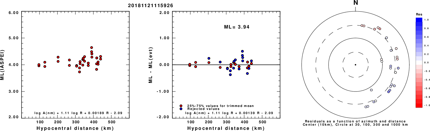
Left: ML computed using the IASPEI formula for Horizontal components. Center: ML residuals computed using a modified IASPEI formula that accounts for path specific attenuation; the values used for the trimmed mean are indicated. The ML relation used for each figure is given at the bottom of each plot.
Right: Residuals from new relation as a function of distance and azimuth.
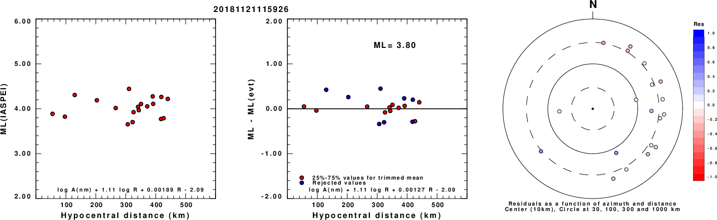
Left: ML computed using the IASPEI formula for Vertical components (research). Center: ML residuals computed using a modified IASPEI formula that accounts for path specific attenuation; the values used for the trimmed mean are indicated. The ML relation used for each figure is given at the bottom of each plot.
Right: Residuals from new relation as a function of distance and azimuth.
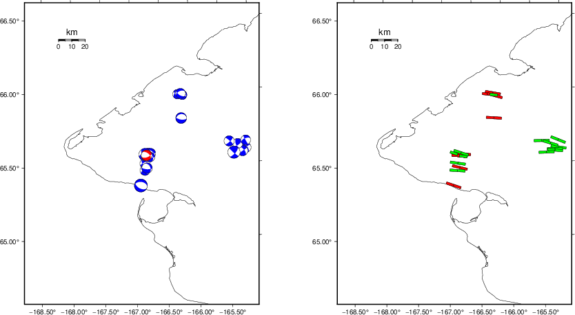 |
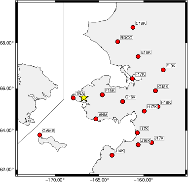
The focal mechanism was determined using broadband seismic waveforms. The location of the event (star) and the stations used for (red) the waveform inversion are shown in the next figure.
|
|
|
The program wvfgrd96 was used with good traces observed at short distance to determine the focal mechanism, depth and seismic moment. This technique requires a high quality signal and well determined velocity model for the Green's functions. To the extent that these are the quality data, this type of mechanism should be preferred over the radiation pattern technique which requires the separate step of defining the pressure and tension quadrants and the correct strike.
The observed and predicted traces are filtered using the following gsac commands:
cut o DIST/3.3 -40 o DIST/3.3 +50
rtr
taper w 0.1
hp c 0.03 n 3
lp c 0.10 n 3
The results of this grid search are as follow:
           DEPTH  STK   DIP  RAKE   MW    FIT
WVFGRD96    1.0   300    85    15   3.37 0.3466
WVFGRD96    2.0   300    80    20   3.49 0.3872
WVFGRD96    3.0   115    80   -15   3.55 0.3606
WVFGRD96    4.0    60    75    55   3.58 0.3751
WVFGRD96    5.0    60    70    50   3.60 0.4345
WVFGRD96    6.0    65    65    50   3.63 0.4805
WVFGRD96    7.0    65    65    45   3.64 0.5131
WVFGRD96    8.0    65    65    50   3.72 0.5282
WVFGRD96    9.0    65    65    50   3.73 0.5436
WVFGRD96   10.0   305    50   -50   3.76 0.5767
WVFGRD96   11.0   305    50   -50   3.78 0.6045
WVFGRD96   12.0   305    50   -50   3.80 0.6248
WVFGRD96   13.0   305    50   -50   3.81 0.6385
WVFGRD96   14.0   310    50   -45   3.83 0.6460
WVFGRD96   15.0   310    50   -45   3.84 0.6490
WVFGRD96   16.0   310    50   -45   3.86 0.6467
WVFGRD96   17.0   310    50   -45   3.87 0.6414
WVFGRD96   18.0   315    50   -40   3.88 0.6331
WVFGRD96   19.0   315    50   -40   3.89 0.6236
WVFGRD96   20.0   315    50   -40   3.90 0.6135
WVFGRD96   21.0   315    50   -40   3.92 0.6034
WVFGRD96   22.0   315    50   -40   3.93 0.5915
WVFGRD96   23.0   315    55   -40   3.93 0.5797
WVFGRD96   24.0   315    55   -40   3.94 0.5675
WVFGRD96   25.0   315    55   -40   3.95 0.5555
WVFGRD96   26.0   320    55   -35   3.95 0.5431
WVFGRD96   27.0   320    55   -35   3.96 0.5299
WVFGRD96   28.0   320    55   -35   3.96 0.5145
WVFGRD96   29.0   135    60   -45   3.95 0.5040
The best solution is
WVFGRD96 15.0 310 50 -45 3.84 0.6490
The mechanism corresponding to the best fit is
|
|
|
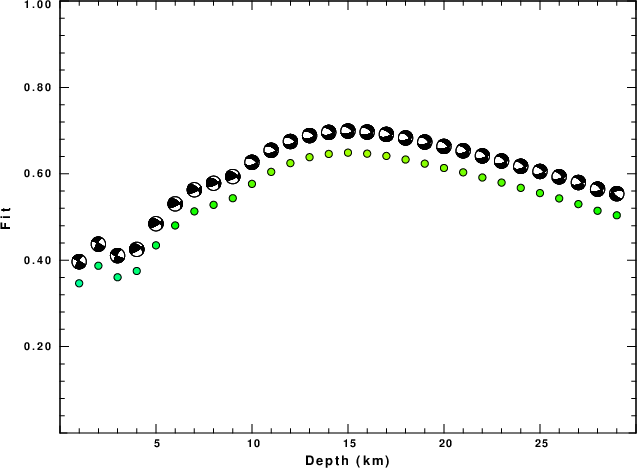
The best fit as a function of depth is given in the following figure:
|
|
|
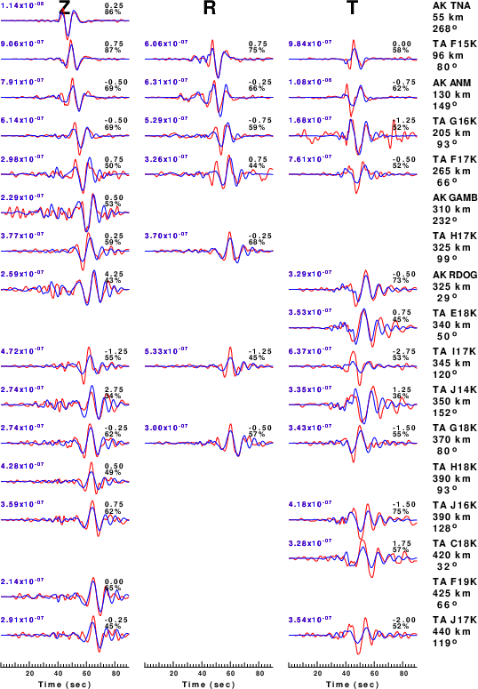
The comparison of the observed and predicted waveforms is given in the next figure. The red traces are the observed and the blue are the predicted. Each observed-predicted component is plotted to the same scale and peak amplitudes are indicated by the numbers to the left of each trace. A pair of numbers is given in black at the right of each predicted traces. The upper number it the time shift required for maximum correlation between the observed and predicted traces. This time shift is required because the synthetics are not computed at exactly the same distance as the observed, the velocity model used in the predictions may not be perfect and the epicentral parameters may be be off. A positive time shift indicates that the prediction is too fast and should be delayed to match the observed trace (shift to the right in this figure). A negative value indicates that the prediction is too slow. The lower number gives the percentage of variance reduction to characterize the individual goodness of fit (100% indicates a perfect fit).
The bandpass filter used in the processing and for the display was
cut o DIST/3.3 -40 o DIST/3.3 +50
rtr
taper w 0.1
hp c 0.03 n 3
lp c 0.10 n 3
|
| Figure 3. Waveform comparison for selected depth. Red: observed; Blue - predicted. The time shift with respect to the model prediction is indicated. The percent of fit is also indicated. The time scale is relative to the first trace sample. |
|
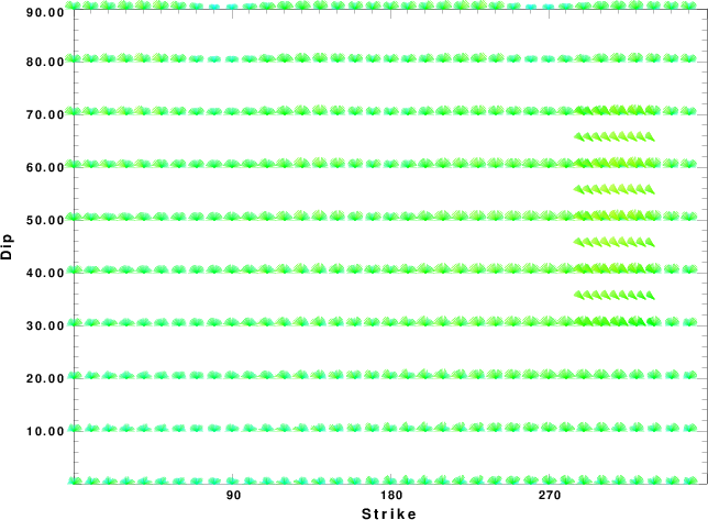
| Focal mechanism sensitivity at the preferred depth. The red color indicates a very good fit to the waveforms. Each solution is plotted as a vector at a given value of strike and dip with the angle of the vector representing the rake angle, measured, with respect to the upward vertical (N) in the figure. |
A check on the assumed source location is possible by looking at the time shifts between the observed and predicted traces. The time shifts for waveform matching arise for several reasons:
Time_shift = A + B cos Azimuth + C Sin Azimuth
The time shifts for this inversion lead to the next figure:
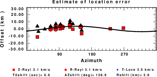
The derived shift in origin time and epicentral coordinates are given at the bottom of the figure.
The WUS.model used for the waveform synthetic seismograms and for the surface wave eigenfunctions and dispersion is as follows (The format is in the model96 format of Computer Programs in Seismology).
MODEL.01
Model after     8 iterations
ISOTROPIC
KGS
FLAT EARTH
1-D
CONSTANT VELOCITY
LINE08
LINE09
LINE10
LINE11
      H(KM)   VP(KM/S)   VS(KM/S) RHO(GM/CC)         QP         QS       ETAP       ETAS      FREFP      FREFS
     1.9000     3.4065     2.0089     2.2150  0.302E-02  0.679E-02   0.00       0.00       1.00       1.00
     6.1000     5.5445     3.2953     2.6089  0.349E-02  0.784E-02   0.00       0.00       1.00       1.00
    13.0000     6.2708     3.7396     2.7812  0.212E-02  0.476E-02   0.00       0.00       1.00       1.00
    19.0000     6.4075     3.7680     2.8223  0.111E-02  0.249E-02   0.00       0.00       1.00       1.00
     0.0000     7.9000     4.6200     3.2760  0.164E-10  0.370E-10   0.00       0.00       1.00       1.00