Location
Location ANSS
The ANSS event ID is ak018by72yh3 and the event page is at
https://earthquake.usgs.gov/earthquakes/eventpage/ak018by72yh3/executive.
2018/09/17 12:35:08 59.708 -153.214 104.8 3.9 Alaska
Focal Mechanism
 USGS/SLU Moment Tensor Solution
 ENS  2018/09/17 12:35:08:0  59.71 -153.21 104.8 3.9 Alaska

 Stations used:
   AT.OHAK AV.ILSW AV.SPU II.KDAK TA.L19K TA.M19K TA.O18K
   TA.P18K TA.Q19K TA.Q20K

 Filtering commands used:
   cut o DIST/3.4 -30 o DIST/3.4 +70
   rtr
   taper w 0.1
   hp c 0.03 n 3
   lp c 0.10 n 3

 Best Fitting Double Couple
  Mo = 9.55e+21 dyne-cm
  Mw = 3.92
  Z  = 118 km
  Plane   Strike  Dip  Rake
   NP1      319    63   127
   NP2       80    45    40
  Principal Axes:
   Axis    Value   Plunge  Azimuth
    T   9.55e+21     55     278
    N   0.00e+00     33     120
    P  -9.55e+21     10      23

 Moment Tensor: (dyne-cm)
    Component   Value
       Mxx    -7.72e+21
       Mxy    -3.81e+21
       Mxz    -8.98e+20
       Myy     1.58e+21
       Myz    -5.09e+21
       Mzz     6.14e+21


                     -------------
                 ----------------- P --
              #-------------------   -----
             ########----------------------
           ##############--------------------
          #################-------------------
         ####################------------------
        #######################-----------------
        #########################---------------
       ###########   ##############-------------#
       ########### T ###############-----------##
       ###########   ################---------###
       ###############################-------####
        ###############################----#####
        --##############################-#######
         ----#########################---######
          -------#################-------#####
           ------------------------------####
             -----------------------------#
              ----------------------------
                 ----------------------
                     --------------


 Global CMT Convention Moment Tensor:
      R          T          P
  6.14e+21  -8.98e+20   5.09e+21
 -8.98e+20  -7.72e+21   3.81e+21
  5.09e+21   3.81e+21   1.58e+21


Details of the solution is found at

http://www.eas.slu.edu/eqc/eqc_mt/MECH.NA/20180917123508/index.html
|
Preferred Solution
The preferred solution from an analysis of the surface-wave spectral amplitude radiation pattern, waveform inversion or first motion observations is
      STK = 80
      DIP = 45
     RAKE = 40
       MW = 3.92
       HS = 118.0
The NDK file is 20180917123508.ndk
The waveform inversion is preferred.
Magnitudes
Given the availability of digital waveforms for determination of the moment tensor, this section documents the added processing leading to mLg, if appropriate to the region, and ML by application of the respective IASPEI formulae. As a research study, the linear distance term of the IASPEI formula
for ML is adjusted to remove a linear distance trend in residuals to give a regionally defined ML. The defined ML uses horizontal component recordings, but the same procedure is applied to the vertical components since there may be some interest in vertical component ground motions. Residual plots versus distance may indicate interesting features of ground motion scaling in some distance ranges. A residual plot of the regionalized magnitude is given as a function of distance and azimuth, since data sets may transcend different wave propagation provinces.
ML Magnitude
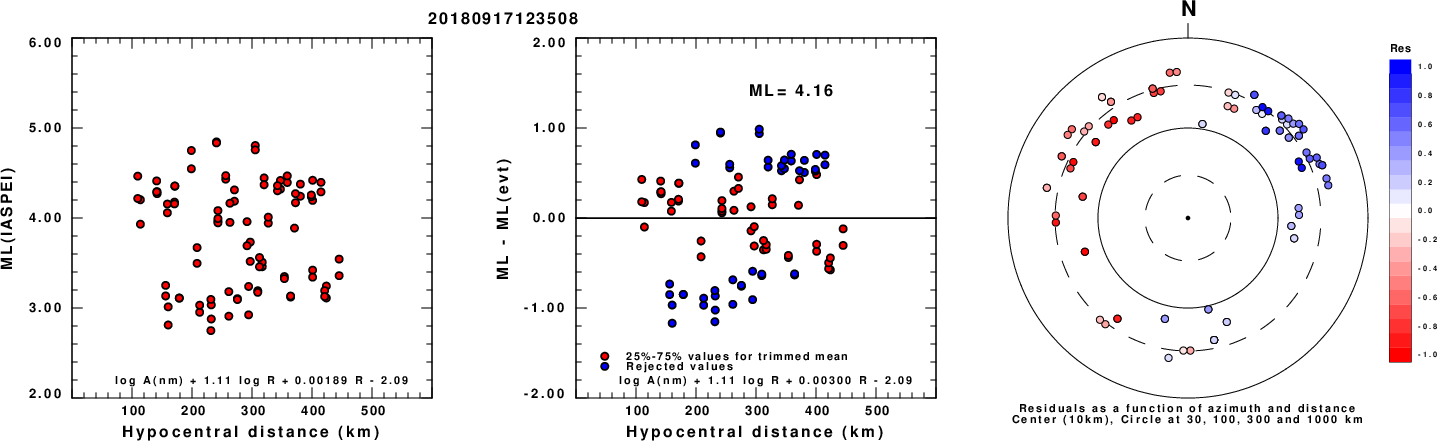
Left: ML computed using the IASPEI formula for Horizontal components. Center: ML residuals computed using a modified IASPEI formula that accounts for path specific attenuation; the values used for the trimmed mean are indicated. The ML relation used for each figure is given at the bottom of each plot.
Right: Residuals from new relation as a function of distance and azimuth.
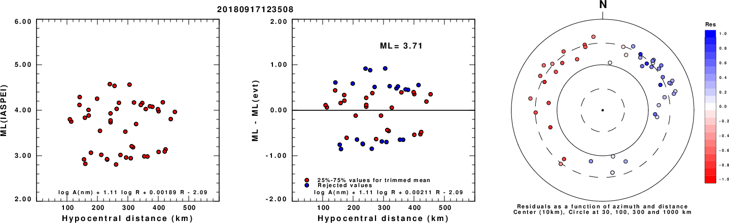
Left: ML computed using the IASPEI formula for Vertical components (research). Center: ML residuals computed using a modified IASPEI formula that accounts for path specific attenuation; the values used for the trimmed mean are indicated. The ML relation used for each figure is given at the bottom of each plot.
Right: Residuals from new relation as a function of distance and azimuth.
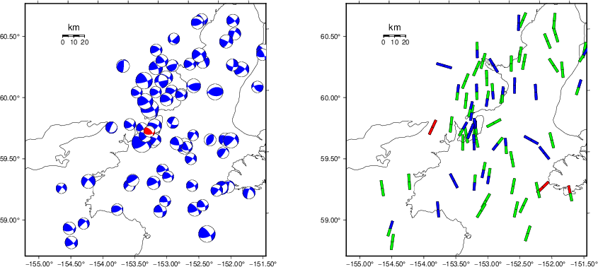
Context
The left panel of the next figure presents the focal mechanism for this earthquake (red) in the context of other nearby events (blue) in the SLU Moment Tensor Catalog. The right panel shows the inferred direction of maximum compressive stress and the type of faulting (green is strike-slip, red is normal, blue is thrust; oblique is shown by a combination of colors). Thus context plot is useful for assessing the appropriateness of the moment tensor of this event.
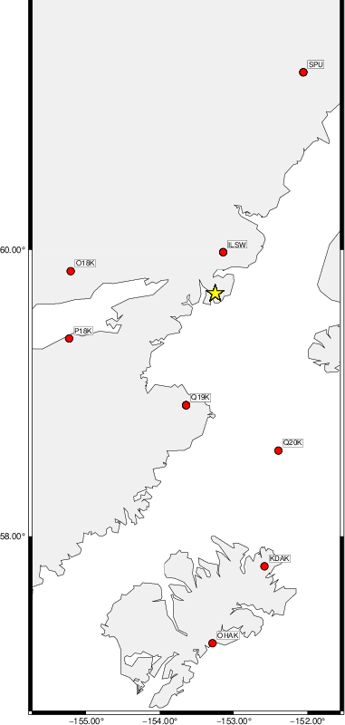
Waveform Inversion using wvfgrd96
The focal mechanism was determined using broadband seismic waveforms. The location of the event (star) and the
stations used for (red) the waveform inversion are shown in the next figure.
|
|
Location of broadband stations used for waveform inversion
|
The program wvfgrd96 was used with good traces observed at short distance to determine the focal mechanism, depth and seismic moment. This technique requires a high quality signal and well determined velocity model for the Green's functions. To the extent that these are the quality data, this type of mechanism should be preferred over the radiation pattern technique which requires the separate step of defining the pressure and tension quadrants and the correct strike.
The observed and predicted traces are filtered using the following gsac commands:
cut o DIST/3.4 -30 o DIST/3.4 +70
rtr
taper w 0.1
hp c 0.03 n 3
lp c 0.10 n 3
The results of this grid search are as follow:
           DEPTH  STK   DIP  RAKE   MW    FIT
WVFGRD96    2.0   330    65   -35   2.96 0.2171
WVFGRD96    4.0   160    85    40   3.08 0.2533
WVFGRD96    6.0   160    85    40   3.16 0.2911
WVFGRD96    8.0   340    90   -50   3.27 0.3149
WVFGRD96   10.0    -5    75    65   3.37 0.3289
WVFGRD96   12.0   185    75    75   3.49 0.3345
WVFGRD96   14.0   185    75    75   3.53 0.3336
WVFGRD96   16.0   230    70    15   3.45 0.3367
WVFGRD96   18.0   230    70    10   3.48 0.3503
WVFGRD96   20.0   230    70    10   3.51 0.3578
WVFGRD96   22.0   230    70    10   3.53 0.3585
WVFGRD96   24.0    70    85    15   3.48 0.3662
WVFGRD96   26.0    75    75    20   3.49 0.3871
WVFGRD96   28.0    75    75    15   3.50 0.4027
WVFGRD96   30.0    65    55   -25   3.60 0.4132
WVFGRD96   32.0    70    65   -15   3.57 0.4210
WVFGRD96   34.0    70    65   -15   3.58 0.4242
WVFGRD96   36.0    70    70   -10   3.59 0.4275
WVFGRD96   38.0    70    75    -5   3.62 0.4316
WVFGRD96   40.0   250    80   -35   3.66 0.4397
WVFGRD96   42.0   250    80   -35   3.68 0.4473
WVFGRD96   44.0   255    90   -35   3.70 0.4540
WVFGRD96   46.0   255    90   -35   3.72 0.4597
WVFGRD96   48.0   255    90   -35   3.74 0.4660
WVFGRD96   50.0   255    90   -35   3.76 0.4731
WVFGRD96   52.0   255    90   -35   3.77 0.4808
WVFGRD96   54.0    75    75    40   3.82 0.4974
WVFGRD96   56.0    75    70    35   3.83 0.5190
WVFGRD96   58.0    75    70    40   3.85 0.5407
WVFGRD96   60.0    75    65    35   3.85 0.5539
WVFGRD96   62.0    75    65    35   3.86 0.5658
WVFGRD96   64.0    75    65    35   3.86 0.5780
WVFGRD96   66.0    75    65    35   3.86 0.5842
WVFGRD96   68.0    75    65    35   3.87 0.5918
WVFGRD96   70.0    75    65    35   3.87 0.5979
WVFGRD96   72.0    75    65    35   3.87 0.6039
WVFGRD96   74.0    75    65    35   3.88 0.6085
WVFGRD96   76.0    75    65    35   3.88 0.6141
WVFGRD96   78.0    75    65    35   3.88 0.6151
WVFGRD96   80.0    75    60    35   3.88 0.6192
WVFGRD96   82.0    75    60    35   3.89 0.6226
WVFGRD96   84.0    80    50    40   3.89 0.6264
WVFGRD96   86.0    80    50    40   3.89 0.6294
WVFGRD96   88.0    80    50    40   3.89 0.6345
WVFGRD96   90.0    80    50    40   3.89 0.6376
WVFGRD96   92.0    80    50    40   3.90 0.6396
WVFGRD96   94.0    80    50    40   3.90 0.6410
WVFGRD96   96.0    80    50    40   3.90 0.6409
WVFGRD96   98.0    80    50    40   3.90 0.6439
WVFGRD96  100.0    80    50    40   3.90 0.6460
WVFGRD96  102.0    80    50    40   3.91 0.6468
WVFGRD96  104.0    80    50    40   3.91 0.6471
WVFGRD96  106.0    80    45    40   3.91 0.6473
WVFGRD96  108.0    80    45    40   3.91 0.6487
WVFGRD96  110.0    80    45    40   3.91 0.6504
WVFGRD96  112.0    80    45    40   3.91 0.6503
WVFGRD96  114.0    80    45    40   3.92 0.6503
WVFGRD96  116.0    80    45    40   3.92 0.6519
WVFGRD96  118.0    80    45    40   3.92 0.6519
WVFGRD96  120.0    80    45    40   3.92 0.6510
WVFGRD96  122.0    80    45    40   3.92 0.6497
WVFGRD96  124.0    80    45    40   3.93 0.6493
WVFGRD96  126.0    80    45    40   3.93 0.6478
WVFGRD96  128.0    75    45    35   3.93 0.6475
WVFGRD96  130.0    75    45    35   3.93 0.6480
WVFGRD96  132.0    75    45    30   3.92 0.6464
WVFGRD96  134.0    75    45    30   3.92 0.6470
WVFGRD96  136.0    75    45    30   3.92 0.6458
WVFGRD96  138.0    75    45    30   3.93 0.6427
WVFGRD96  140.0    75    45    30   3.93 0.6421
WVFGRD96  142.0    75    45    30   3.93 0.6411
WVFGRD96  144.0    75    45    30   3.93 0.6416
WVFGRD96  146.0    75    45    30   3.93 0.6395
WVFGRD96  148.0    75    45    30   3.94 0.6360
The best solution is
WVFGRD96 118.0 80 45 40 3.92 0.6519
The mechanism corresponding to the best fit is
|
|
Figure 1. Waveform inversion focal mechanism
|
The best fit as a function of depth is given in the following figure:
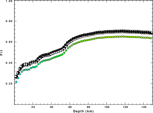
|
|
Figure 2. Depth sensitivity for waveform mechanism
|
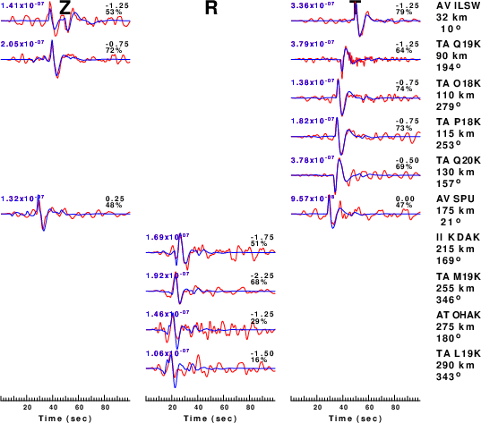
The comparison of the observed and predicted waveforms is given in the next figure. The red traces are the observed and the blue are the predicted.
Each observed-predicted component is plotted to the same scale and peak amplitudes are indicated by the numbers to the left of each trace. A pair of numbers is given in black at the right of each predicted traces. The upper number it the time shift required for maximum correlation between the observed and predicted traces. This time shift is required because the synthetics are not computed at exactly the same distance as the observed, the velocity model used in the predictions may not be perfect and the epicentral parameters may be be off.
A positive time shift indicates that the prediction is too fast and should be delayed to match the observed trace (shift to the right in this figure). A negative value indicates that the prediction is too slow. The lower number gives the percentage of variance reduction to characterize the individual goodness of fit (100% indicates a perfect fit).
The bandpass filter used in the processing and for the display was
cut o DIST/3.4 -30 o DIST/3.4 +70
rtr
taper w 0.1
hp c 0.03 n 3
lp c 0.10 n 3
|
|
Figure 3. Waveform comparison for selected depth. Red: observed; Blue - predicted. The time shift with respect to the model prediction is indicated. The percent of fit is also indicated. The time scale is relative to the first trace sample.
|
|
|
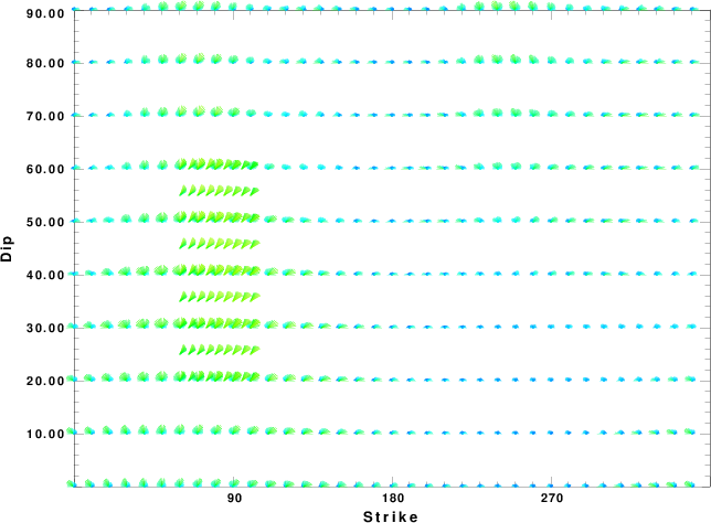
Focal mechanism sensitivity at the preferred depth. The red color indicates a very good fit to the waveforms.
Each solution is plotted as a vector at a given value of strike and dip with the angle of the vector representing the rake angle, measured, with respect to the upward vertical (N) in the figure.
|
A check on the assumed source location is possible by looking at the time shifts between the observed and predicted traces. The time shifts for waveform matching arise for several reasons:
- The origin time and epicentral distance are incorrect
- The velocity model used for the inversion is incorrect
- The velocity model used to define the P-arrival time is not the
same as the velocity model used for the waveform inversion
(assuming that the initial trace alignment is based on the
P arrival time)
Assuming only a mislocation, the time shifts are fit to a functional form:
Time_shift = A + B cos Azimuth + C Sin Azimuth
The time shifts for this inversion lead to the next figure:
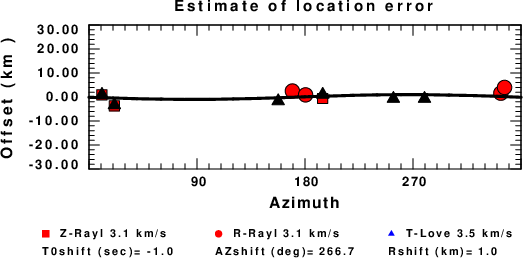
The derived shift in origin time and epicentral coordinates are given at the bottom of the figure.
Velocity Model
The WUS.model used for the waveform synthetic seismograms and for the surface wave eigenfunctions and dispersion is as follows
(The format is in the model96 format of Computer Programs in Seismology).
MODEL.01
Model after     8 iterations
ISOTROPIC
KGS
FLAT EARTH
1-D
CONSTANT VELOCITY
LINE08
LINE09
LINE10
LINE11
      H(KM)   VP(KM/S)   VS(KM/S) RHO(GM/CC)         QP         QS       ETAP       ETAS      FREFP      FREFS
     1.9000     3.4065     2.0089     2.2150  0.302E-02  0.679E-02   0.00       0.00       1.00       1.00
     6.1000     5.5445     3.2953     2.6089  0.349E-02  0.784E-02   0.00       0.00       1.00       1.00
    13.0000     6.2708     3.7396     2.7812  0.212E-02  0.476E-02   0.00       0.00       1.00       1.00
    19.0000     6.4075     3.7680     2.8223  0.111E-02  0.249E-02   0.00       0.00       1.00       1.00
     0.0000     7.9000     4.6200     3.2760  0.164E-10  0.370E-10   0.00       0.00       1.00       1.00
Last Changed Fri Apr 26 02:35:12 AM CDT 2024