Location
Location ANSS
The ANSS event ID is ak0188d4oyaj and the event page is at
https://earthquake.usgs.gov/earthquakes/eventpage/ak0188d4oyaj/executive.
2018/07/01 08:20:16 63.068 -150.797 117.3 5 Alaska
Focal Mechanism
 USGS/SLU Moment Tensor Solution
 ENS  2018/07/01 08:20:16:0  63.07 -150.80 117.3 5.0 Alaska

 Stations used:
   AK.BPAW AK.BWN AK.CAPN AK.CAST AK.CCB AK.CUT AK.DHY AK.DIV
   AK.FID AK.GHO AK.GLB AK.GLI AK.HDA AK.HIN AK.KLU AK.KNK
   AK.KTH AK.MCK AK.MLY AK.NEA2 AK.PAX AK.PPLA AK.RC01 AK.RND
   AK.SAW AK.SCM AK.SCRK AK.SKN AK.SSN AK.WRH AT.PMR AT.SVW2
   AV.SPU IM.IL31 IU.COLA TA.H21K TA.H24K TA.I20K TA.I23K
   TA.J18K TA.J19K TA.J20K TA.J25K TA.L18K TA.L19K TA.M19K
   TA.M22K TA.M24K TA.N19K TA.POKR

 Filtering commands used:
   cut o DIST/3.7 -50 o DIST/3.7 +50
   rtr
   taper w 0.1
   hp c 0.03 n 3
   lp c 0.10 n 3

 Best Fitting Double Couple
  Mo = 2.54e+23 dyne-cm
  Mw = 4.87
  Z  = 126 km
  Plane   Strike  Dip  Rake
   NP1      193    78   -112
   NP2       75    25   -30
  Principal Axes:
   Axis    Value   Plunge  Azimuth
    T   2.54e+23     29     300
    N   0.00e+00     21     197
    P  -2.54e+23     52      77

 Moment Tensor: (dyne-cm)
    Component   Value
       Mxx     4.43e+22
       Mxy    -1.05e+23
       Mxz     2.73e+22
       Myy     5.30e+22
       Myz    -2.14e+23
       Mzz    -9.73e+22


                     ###########---
                 ##############--------
              ################------------
             ################--------------
           #################-----------------
          ####   ###########------------------
         ##### T ##########--------------------
        ######   #########----------------------
        ##################----------   ---------
       ##################----------- P ---------#
       ##################-----------   ---------#
       ##################----------------------##
       #################-----------------------##
        ################----------------------##
        -###############---------------------###
         -#############--------------------####
          --###########------------------#####
           ---#########----------------######
             ----######-------------#######
              ----------------############
                 ------################
                     --############


 Global CMT Convention Moment Tensor:
      R          T          P
 -9.73e+22   2.73e+22   2.14e+23
  2.73e+22   4.43e+22   1.05e+23
  2.14e+23   1.05e+23   5.30e+22


Details of the solution is found at

http://www.eas.slu.edu/eqc/eqc_mt/MECH.NA/20180701082016/index.html
|
Preferred Solution
The preferred solution from an analysis of the surface-wave spectral amplitude radiation pattern, waveform inversion or first motion observations is
      STK = 75
      DIP = 25
     RAKE = -30
       MW = 4.87
       HS = 126.0
The NDK file is 20180701082016.ndk
The waveform inversion is preferred.
Magnitudes
Given the availability of digital waveforms for determination of the moment tensor, this section documents the added processing leading to mLg, if appropriate to the region, and ML by application of the respective IASPEI formulae. As a research study, the linear distance term of the IASPEI formula
for ML is adjusted to remove a linear distance trend in residuals to give a regionally defined ML. The defined ML uses horizontal component recordings, but the same procedure is applied to the vertical components since there may be some interest in vertical component ground motions. Residual plots versus distance may indicate interesting features of ground motion scaling in some distance ranges. A residual plot of the regionalized magnitude is given as a function of distance and azimuth, since data sets may transcend different wave propagation provinces.
ML Magnitude
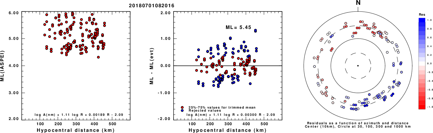
Left: ML computed using the IASPEI formula for Horizontal components. Center: ML residuals computed using a modified IASPEI formula that accounts for path specific attenuation; the values used for the trimmed mean are indicated. The ML relation used for each figure is given at the bottom of each plot.
Right: Residuals from new relation as a function of distance and azimuth.
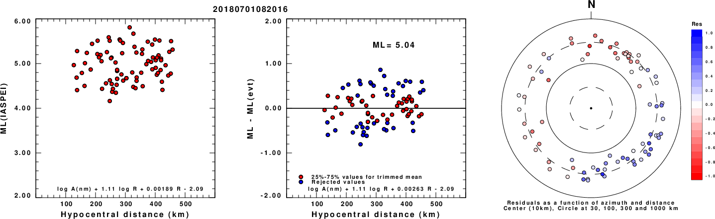
Left: ML computed using the IASPEI formula for Vertical components (research). Center: ML residuals computed using a modified IASPEI formula that accounts for path specific attenuation; the values used for the trimmed mean are indicated. The ML relation used for each figure is given at the bottom of each plot.
Right: Residuals from new relation as a function of distance and azimuth.
Context
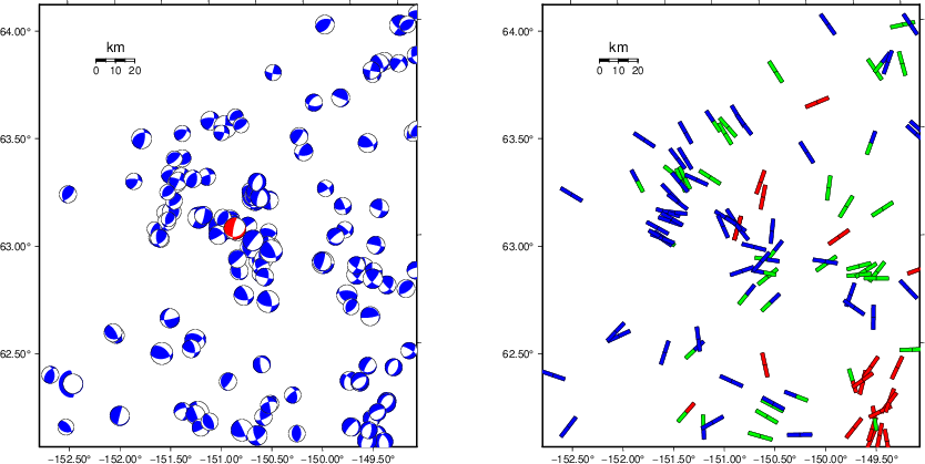
The left panel of the next figure presents the focal mechanism for this earthquake (red) in the context of other nearby events (blue) in the SLU Moment Tensor Catalog. The right panel shows the inferred direction of maximum compressive stress and the type of faulting (green is strike-slip, red is normal, blue is thrust; oblique is shown by a combination of colors). Thus context plot is useful for assessing the appropriateness of the moment tensor of this event.
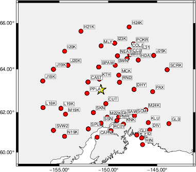
Waveform Inversion using wvfgrd96
The focal mechanism was determined using broadband seismic waveforms. The location of the event (star) and the
stations used for (red) the waveform inversion are shown in the next figure.
|
|
Location of broadband stations used for waveform inversion
|
The program wvfgrd96 was used with good traces observed at short distance to determine the focal mechanism, depth and seismic moment. This technique requires a high quality signal and well determined velocity model for the Green's functions. To the extent that these are the quality data, this type of mechanism should be preferred over the radiation pattern technique which requires the separate step of defining the pressure and tension quadrants and the correct strike.
The observed and predicted traces are filtered using the following gsac commands:
cut o DIST/3.7 -50 o DIST/3.7 +50
rtr
taper w 0.1
hp c 0.03 n 3
lp c 0.10 n 3
The results of this grid search are as follow:
           DEPTH  STK   DIP  RAKE   MW    FIT
WVFGRD96    2.0     0    85     5   3.81 0.1612
WVFGRD96    4.0   180    70     5   3.93 0.1852
WVFGRD96    6.0   180    70    10   4.00 0.2003
WVFGRD96    8.0   180    70    10   4.08 0.2149
WVFGRD96   10.0   175    75   -15   4.13 0.2221
WVFGRD96   12.0   175    75   -10   4.17 0.2238
WVFGRD96   14.0     0    80    10   4.20 0.2181
WVFGRD96   16.0     0    80    10   4.23 0.2110
WVFGRD96   18.0   270    85    15   4.25 0.2109
WVFGRD96   20.0   270    90    15   4.27 0.2153
WVFGRD96   22.0   270    70    10   4.30 0.2236
WVFGRD96   24.0   270    85    15   4.32 0.2334
WVFGRD96   26.0    90    85   -15   4.35 0.2466
WVFGRD96   28.0    90    85   -15   4.37 0.2600
WVFGRD96   30.0    90    80   -15   4.39 0.2723
WVFGRD96   32.0    90    85   -15   4.41 0.2834
WVFGRD96   34.0    90    80   -15   4.43 0.2935
WVFGRD96   36.0    90    80   -15   4.45 0.2997
WVFGRD96   38.0    90    80   -10   4.48 0.3026
WVFGRD96   40.0    90    80   -15   4.53 0.3038
WVFGRD96   42.0    90    75   -10   4.56 0.3021
WVFGRD96   44.0    85    70   -15   4.58 0.3031
WVFGRD96   46.0    85    70   -15   4.60 0.3059
WVFGRD96   48.0    85    70   -15   4.61 0.3091
WVFGRD96   50.0    85    70   -15   4.63 0.3141
WVFGRD96   52.0    85    65   -15   4.65 0.3202
WVFGRD96   54.0    95    60    15   4.68 0.3288
WVFGRD96   56.0    95    60    15   4.69 0.3363
WVFGRD96   58.0    95    60    10   4.70 0.3461
WVFGRD96   60.0    90    60    10   4.70 0.3540
WVFGRD96   62.0    90    60     5   4.70 0.3619
WVFGRD96   64.0    90    60     5   4.71 0.3691
WVFGRD96   66.0    90    60     5   4.72 0.3774
WVFGRD96   68.0    85    60   -10   4.72 0.3838
WVFGRD96   70.0    85    30   -15   4.76 0.3965
WVFGRD96   72.0    85    30   -15   4.77 0.4111
WVFGRD96   74.0    85    30   -15   4.77 0.4246
WVFGRD96   76.0    85    30   -15   4.78 0.4371
WVFGRD96   78.0    85    30   -15   4.79 0.4515
WVFGRD96   80.0    80    30   -20   4.79 0.4637
WVFGRD96   82.0    75    20   -25   4.81 0.4766
WVFGRD96   84.0    80    20   -20   4.81 0.4910
WVFGRD96   86.0    75    20   -25   4.82 0.5054
WVFGRD96   88.0    75    20   -25   4.82 0.5174
WVFGRD96   90.0    75    20   -25   4.83 0.5282
WVFGRD96   92.0    75    20   -25   4.83 0.5369
WVFGRD96   94.0    80    20   -25   4.84 0.5459
WVFGRD96   96.0    80    20   -25   4.84 0.5542
WVFGRD96   98.0    80    20   -25   4.85 0.5608
WVFGRD96  100.0    75    20   -30   4.85 0.5666
WVFGRD96  102.0    75    20   -30   4.85 0.5719
WVFGRD96  104.0    75    20   -30   4.85 0.5768
WVFGRD96  106.0    75    20   -30   4.86 0.5795
WVFGRD96  108.0    75    20   -30   4.86 0.5827
WVFGRD96  110.0    75    20   -30   4.86 0.5854
WVFGRD96  112.0    75    25   -30   4.86 0.5884
WVFGRD96  114.0    75    25   -30   4.86 0.5916
WVFGRD96  116.0    75    25   -30   4.86 0.5955
WVFGRD96  118.0    75    25   -30   4.86 0.5965
WVFGRD96  120.0    75    25   -30   4.86 0.5998
WVFGRD96  122.0    75    25   -30   4.87 0.6001
WVFGRD96  124.0    75    25   -30   4.87 0.6011
WVFGRD96  126.0    75    25   -30   4.87 0.6024
WVFGRD96  128.0    75    25   -30   4.87 0.6003
WVFGRD96  130.0    75    25   -30   4.87 0.6010
WVFGRD96  132.0    75    25   -30   4.87 0.5988
WVFGRD96  134.0    75    25   -30   4.87 0.5994
WVFGRD96  136.0    75    25   -30   4.87 0.5968
WVFGRD96  138.0    75    25   -30   4.87 0.5961
WVFGRD96  140.0    75    25   -30   4.88 0.5941
WVFGRD96  142.0    75    25   -35   4.88 0.5912
WVFGRD96  144.0    75    25   -35   4.88 0.5903
WVFGRD96  146.0    75    25   -35   4.88 0.5867
WVFGRD96  148.0    85    25   -25   4.89 0.5847
The best solution is
WVFGRD96 126.0 75 25 -30 4.87 0.6024
The mechanism corresponding to the best fit is
|
|
Figure 1. Waveform inversion focal mechanism
|
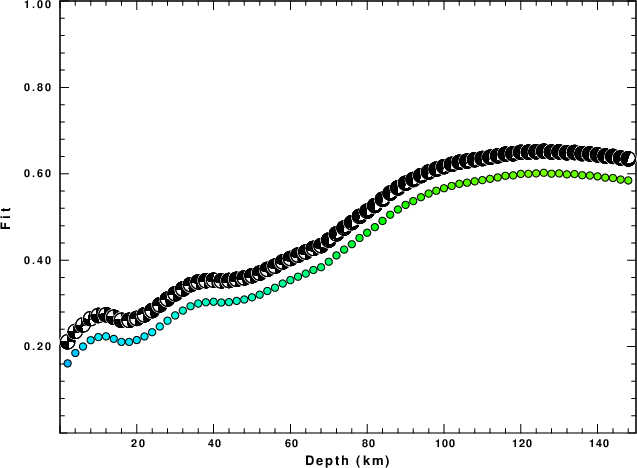
The best fit as a function of depth is given in the following figure:
|
|
Figure 2. Depth sensitivity for waveform mechanism
|
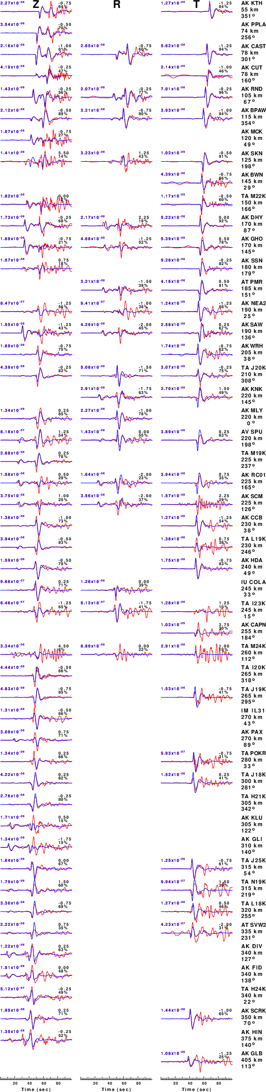
The comparison of the observed and predicted waveforms is given in the next figure. The red traces are the observed and the blue are the predicted.
Each observed-predicted component is plotted to the same scale and peak amplitudes are indicated by the numbers to the left of each trace. A pair of numbers is given in black at the right of each predicted traces. The upper number it the time shift required for maximum correlation between the observed and predicted traces. This time shift is required because the synthetics are not computed at exactly the same distance as the observed, the velocity model used in the predictions may not be perfect and the epicentral parameters may be be off.
A positive time shift indicates that the prediction is too fast and should be delayed to match the observed trace (shift to the right in this figure). A negative value indicates that the prediction is too slow. The lower number gives the percentage of variance reduction to characterize the individual goodness of fit (100% indicates a perfect fit).
The bandpass filter used in the processing and for the display was
cut o DIST/3.7 -50 o DIST/3.7 +50
rtr
taper w 0.1
hp c 0.03 n 3
lp c 0.10 n 3
|
|
Figure 3. Waveform comparison for selected depth. Red: observed; Blue - predicted. The time shift with respect to the model prediction is indicated. The percent of fit is also indicated. The time scale is relative to the first trace sample.
|
|
|
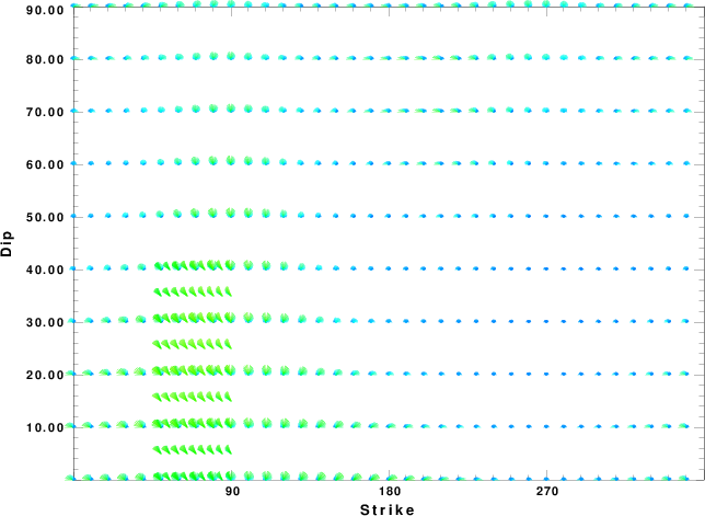
Focal mechanism sensitivity at the preferred depth. The red color indicates a very good fit to the waveforms.
Each solution is plotted as a vector at a given value of strike and dip with the angle of the vector representing the rake angle, measured, with respect to the upward vertical (N) in the figure.
|
A check on the assumed source location is possible by looking at the time shifts between the observed and predicted traces. The time shifts for waveform matching arise for several reasons:
- The origin time and epicentral distance are incorrect
- The velocity model used for the inversion is incorrect
- The velocity model used to define the P-arrival time is not the
same as the velocity model used for the waveform inversion
(assuming that the initial trace alignment is based on the
P arrival time)
Assuming only a mislocation, the time shifts are fit to a functional form:
Time_shift = A + B cos Azimuth + C Sin Azimuth
The time shifts for this inversion lead to the next figure:
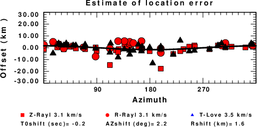
The derived shift in origin time and epicentral coordinates are given at the bottom of the figure.
Velocity Model
The WUS.model used for the waveform synthetic seismograms and for the surface wave eigenfunctions and dispersion is as follows
(The format is in the model96 format of Computer Programs in Seismology).
MODEL.01
Model after     8 iterations
ISOTROPIC
KGS
FLAT EARTH
1-D
CONSTANT VELOCITY
LINE08
LINE09
LINE10
LINE11
      H(KM)   VP(KM/S)   VS(KM/S) RHO(GM/CC)         QP         QS       ETAP       ETAS      FREFP      FREFS
     1.9000     3.4065     2.0089     2.2150  0.302E-02  0.679E-02   0.00       0.00       1.00       1.00
     6.1000     5.5445     3.2953     2.6089  0.349E-02  0.784E-02   0.00       0.00       1.00       1.00
    13.0000     6.2708     3.7396     2.7812  0.212E-02  0.476E-02   0.00       0.00       1.00       1.00
    19.0000     6.4075     3.7680     2.8223  0.111E-02  0.249E-02   0.00       0.00       1.00       1.00
     0.0000     7.9000     4.6200     3.2760  0.164E-10  0.370E-10   0.00       0.00       1.00       1.00
Last Changed Fri Apr 26 12:01:22 AM CDT 2024