Location
SLU Location
Because the initial ANSS location of 57 km is much less than the
moment tensor depth, first arrivals were hand picked and the
event located with the WUS model given below. The output of
elocate is given in elocate.txt. Although the WUS model
is not appropriate for this region, the SLU depth of 88 km is much closer to the RMT depth of 108 km than the initial 57 km depth.. in addition
the first motions selected agree well with the RMT nodal planes.
Location ANSS
The ANSS event ID is ak0187uygjsf and the event page is at
https://earthquake.usgs.gov/earthquakes/eventpage/ak0187uygjsf/executive.
2018/06/20 09:34:08 63.305 -148.123 71.9 3.7 Alaska
Focal Mechanism
 USGS/SLU Moment Tensor Solution
 ENS  2018/06/20 09:34:08:0  63.31 -148.12  71.9 3.7 Alaska

 Stations used:
   AK.BPAW AK.CAST AK.CUT AK.HDA AK.KLU AK.KNK AK.KTH AK.MCK
   AK.NEA2 AK.PAX AK.RND AK.SAW AK.SCM AK.SKN AK.SSN AK.WRH
   IM.IL31 IU.COLA TA.J25K TA.J26L TA.M22K TA.M24K TA.N25K

 Filtering commands used:
   cut o DIST/3.3 -50 o DIST/3.3 +30
   rtr
   taper w 0.1
   hp c 0.03 n 3
   lp c 0.10 n 3

 Best Fitting Double Couple
  Mo = 1.02e+22 dyne-cm
  Mw = 3.94
  Z  = 108 km
  Plane   Strike  Dip  Rake
   NP1      150    75    25
   NP2       53    66   164
  Principal Axes:
   Axis    Value   Plunge  Azimuth
    T   1.02e+22     28      13
    N   0.00e+00     61     179
    P  -1.02e+22      6     280

 Moment Tensor: (dyne-cm)
    Component   Value
       Mxx     7.22e+21
       Mxy     3.54e+21
       Mxz     3.95e+21
       Myy    -9.38e+21
       Myz     2.04e+21
       Mzz     2.16e+21


                     ##############
                 -#####################
              ----############   #########
             -----############ T ##########
           --------###########   ############
          ---------#########################--
         -----------#######################----
        -------------#####################------
          -----------####################-------
        P ------------##################---------
          -------------###############-----------
       -----------------############-------------
       ------------------#########---------------
        ------------------######----------------
        --------------------#-------------------
         -----------------###------------------
          -------------#######----------------
           ------###############-------------
             ####################----------
              #####################-------
                 #####################-
                     ##############


 Global CMT Convention Moment Tensor:
      R          T          P
  2.16e+21   3.95e+21  -2.04e+21
  3.95e+21   7.22e+21  -3.54e+21
 -2.04e+21  -3.54e+21  -9.38e+21


Details of the solution is found at

http://www.eas.slu.edu/eqc/eqc_mt/MECH.NA/20180620093408/index.html
|
Preferred Solution
The preferred solution from an analysis of the surface-wave spectral amplitude radiation pattern, waveform inversion or first motion observations is
      STK = 150
      DIP = 75
     RAKE = 25
       MW = 3.94
       HS = 108.0
The NDK file is 20180620093408.ndk
The waveform inversion is preferred.
Moment Tensor Comparison
The following compares this source inversion to those provided by others. The purpose is to look for major differences and also to note slight differences that might be inherent to the processing procedure. For completeness the USGS/SLU solution is repeated from above.
| SLU |
SLUFM |
 USGS/SLU Moment Tensor Solution
 ENS  2018/06/20 09:34:08:0  63.31 -148.12  71.9 3.7 Alaska

 Stations used:
   AK.BPAW AK.CAST AK.CUT AK.HDA AK.KLU AK.KNK AK.KTH AK.MCK
   AK.NEA2 AK.PAX AK.RND AK.SAW AK.SCM AK.SKN AK.SSN AK.WRH
   IM.IL31 IU.COLA TA.J25K TA.J26L TA.M22K TA.M24K TA.N25K

 Filtering commands used:
   cut o DIST/3.3 -50 o DIST/3.3 +30
   rtr
   taper w 0.1
   hp c 0.03 n 3
   lp c 0.10 n 3

 Best Fitting Double Couple
  Mo = 1.02e+22 dyne-cm
  Mw = 3.94
  Z  = 108 km
  Plane   Strike  Dip  Rake
   NP1      150    75    25
   NP2       53    66   164
  Principal Axes:
   Axis    Value   Plunge  Azimuth
    T   1.02e+22     28      13
    N   0.00e+00     61     179
    P  -1.02e+22      6     280

 Moment Tensor: (dyne-cm)
    Component   Value
       Mxx     7.22e+21
       Mxy     3.54e+21
       Mxz     3.95e+21
       Myy    -9.38e+21
       Myz     2.04e+21
       Mzz     2.16e+21


                     ##############
                 -#####################
              ----############   #########
             -----############ T ##########
           --------###########   ############
          ---------#########################--
         -----------#######################----
        -------------#####################------
          -----------####################-------
        P ------------##################---------
          -------------###############-----------
       -----------------############-------------
       ------------------#########---------------
        ------------------######----------------
        --------------------#-------------------
         -----------------###------------------
          -------------#######----------------
           ------###############-------------
             ####################----------
              #####################-------
                 #####################-
                     ##############


 Global CMT Convention Moment Tensor:
      R          T          P
  2.16e+21   3.95e+21  -2.04e+21
  3.95e+21   7.22e+21  -3.54e+21
 -2.04e+21  -3.54e+21  -9.38e+21


Details of the solution is found at

http://www.eas.slu.edu/eqc/eqc_mt/MECH.NA/20180620093408/index.html
|
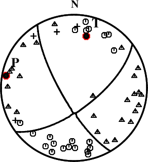
First motions and takeoff angles from an elocate run.
|
Magnitudes
Given the availability of digital waveforms for determination of the moment tensor, this section documents the added processing leading to mLg, if appropriate to the region, and ML by application of the respective IASPEI formulae. As a research study, the linear distance term of the IASPEI formula
for ML is adjusted to remove a linear distance trend in residuals to give a regionally defined ML. The defined ML uses horizontal component recordings, but the same procedure is applied to the vertical components since there may be some interest in vertical component ground motions. Residual plots versus distance may indicate interesting features of ground motion scaling in some distance ranges. A residual plot of the regionalized magnitude is given as a function of distance and azimuth, since data sets may transcend different wave propagation provinces.
ML Magnitude
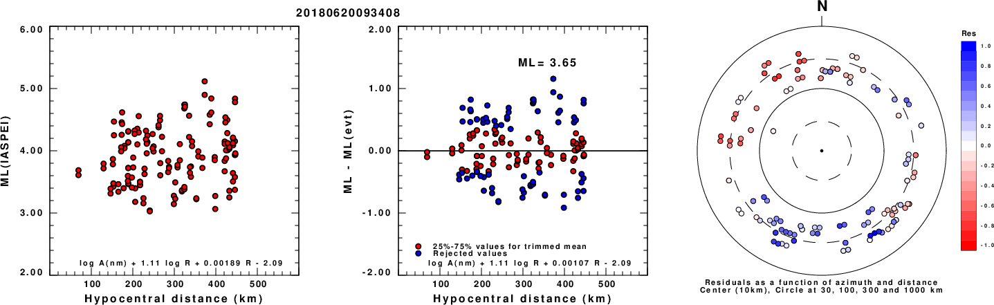
Left: ML computed using the IASPEI formula for Horizontal components. Center: ML residuals computed using a modified IASPEI formula that accounts for path specific attenuation; the values used for the trimmed mean are indicated. The ML relation used for each figure is given at the bottom of each plot.
Right: Residuals from new relation as a function of distance and azimuth.
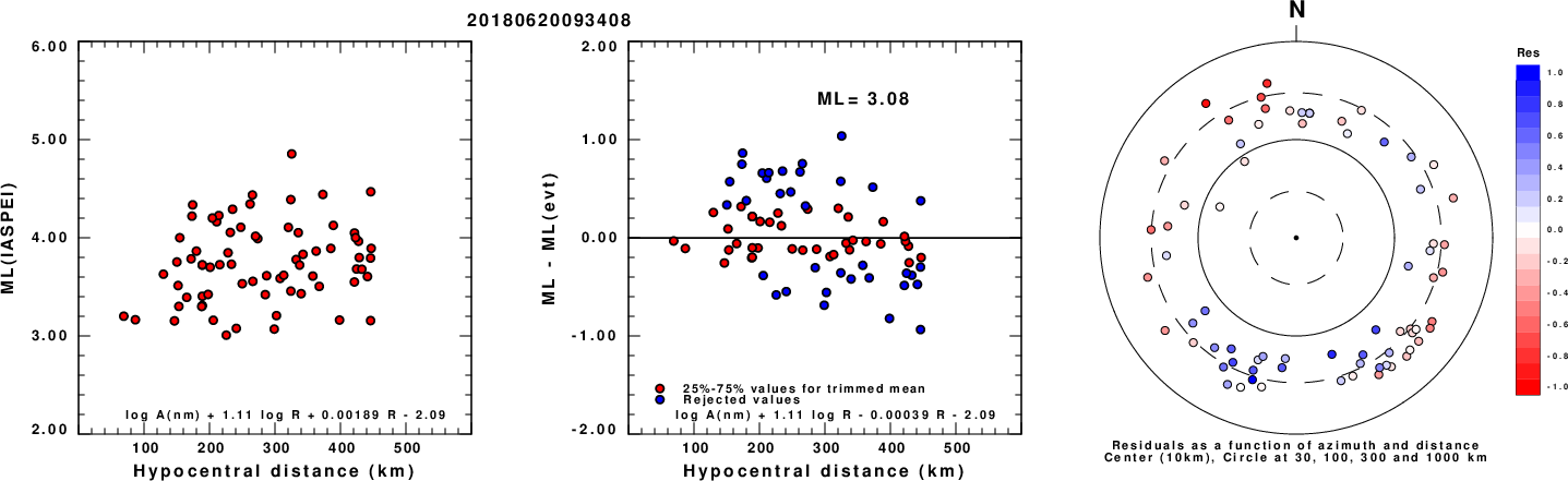
Left: ML computed using the IASPEI formula for Vertical components (research). Center: ML residuals computed using a modified IASPEI formula that accounts for path specific attenuation; the values used for the trimmed mean are indicated. The ML relation used for each figure is given at the bottom of each plot.
Right: Residuals from new relation as a function of distance and azimuth.
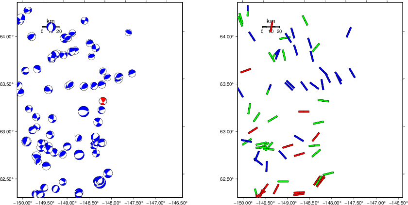
Context
The left panel of the next figure presents the focal mechanism for this earthquake (red) in the context of other nearby events (blue) in the SLU Moment Tensor Catalog. The right panel shows the inferred direction of maximum compressive stress and the type of faulting (green is strike-slip, red is normal, blue is thrust; oblique is shown by a combination of colors). Thus context plot is useful for assessing the appropriateness of the moment tensor of this event.
Waveform Inversion using wvfgrd96
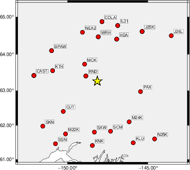
The focal mechanism was determined using broadband seismic waveforms. The location of the event (star) and the
stations used for (red) the waveform inversion are shown in the next figure.
|
|
Location of broadband stations used for waveform inversion
|
The program wvfgrd96 was used with good traces observed at short distance to determine the focal mechanism, depth and seismic moment. This technique requires a high quality signal and well determined velocity model for the Green's functions. To the extent that these are the quality data, this type of mechanism should be preferred over the radiation pattern technique which requires the separate step of defining the pressure and tension quadrants and the correct strike.
The observed and predicted traces are filtered using the following gsac commands:
cut o DIST/3.3 -50 o DIST/3.3 +30
rtr
taper w 0.1
hp c 0.03 n 3
lp c 0.10 n 3
The results of this grid search are as follow:
           DEPTH  STK   DIP  RAKE   MW    FIT
WVFGRD96    2.0   240    85     0   2.95 0.1370
WVFGRD96    4.0   240    65    10   3.07 0.1603
WVFGRD96    6.0   240    70    10   3.12 0.1727
WVFGRD96    8.0   240    70    10   3.20 0.1797
WVFGRD96   10.0   240    70     5   3.24 0.1824
WVFGRD96   12.0   240    70     5   3.27 0.1799
WVFGRD96   14.0   140    85   -25   3.31 0.1886
WVFGRD96   16.0   325    85    25   3.35 0.1998
WVFGRD96   18.0   140    90   -25   3.38 0.2069
WVFGRD96   20.0   325    80    20   3.42 0.2133
WVFGRD96   22.0   325    80    20   3.45 0.2187
WVFGRD96   24.0   330    80    15   3.47 0.2234
WVFGRD96   26.0   330    75    15   3.49 0.2262
WVFGRD96   28.0   330    75    20   3.51 0.2270
WVFGRD96   30.0   330    75    15   3.53 0.2319
WVFGRD96   32.0   330    75    15   3.55 0.2364
WVFGRD96   34.0   330    75    15   3.58 0.2416
WVFGRD96   36.0   330    75    10   3.60 0.2475
WVFGRD96   38.0   330    75    10   3.64 0.2581
WVFGRD96   40.0   330    75    10   3.70 0.2773
WVFGRD96   42.0   330    75     5   3.73 0.2862
WVFGRD96   44.0   330    75    10   3.76 0.2909
WVFGRD96   46.0   330    80     5   3.78 0.2960
WVFGRD96   48.0   330    80     0   3.80 0.3019
WVFGRD96   50.0   330    80     0   3.82 0.3093
WVFGRD96   52.0   330    80    -5   3.84 0.3196
WVFGRD96   54.0   330    80    -5   3.85 0.3300
WVFGRD96   56.0   330    80    -5   3.86 0.3423
WVFGRD96   58.0   330    80    -5   3.87 0.3545
WVFGRD96   60.0   150    90    10   3.87 0.3645
WVFGRD96   62.0   330    85   -10   3.89 0.3757
WVFGRD96   64.0   150    90    15   3.89 0.3858
WVFGRD96   66.0   330    90   -10   3.89 0.3953
WVFGRD96   68.0   150    90    15   3.90 0.4029
WVFGRD96   70.0   150    85    15   3.90 0.4098
WVFGRD96   72.0   330    90   -15   3.90 0.4169
WVFGRD96   74.0   150    85    15   3.90 0.4230
WVFGRD96   76.0   150    85    20   3.91 0.4287
WVFGRD96   78.0   150    80    20   3.91 0.4338
WVFGRD96   80.0   150    80    20   3.91 0.4374
WVFGRD96   82.0   150    80    20   3.91 0.4418
WVFGRD96   84.0   150    80    25   3.92 0.4442
WVFGRD96   86.0   150    80    25   3.92 0.4471
WVFGRD96   88.0   150    80    25   3.92 0.4498
WVFGRD96   90.0   150    80    25   3.93 0.4508
WVFGRD96   92.0   150    80    25   3.93 0.4535
WVFGRD96   94.0   150    80    25   3.93 0.4555
WVFGRD96   96.0   150    75    25   3.93 0.4561
WVFGRD96   98.0   150    75    25   3.93 0.4573
WVFGRD96  100.0   150    75    25   3.94 0.4592
WVFGRD96  102.0   150    75    25   3.94 0.4593
WVFGRD96  104.0   150    75    25   3.94 0.4598
WVFGRD96  106.0   150    75    25   3.94 0.4600
WVFGRD96  108.0   150    75    25   3.94 0.4607
WVFGRD96  110.0   150    75    25   3.94 0.4605
WVFGRD96  112.0   150    75    25   3.95 0.4596
WVFGRD96  114.0   150    75    25   3.95 0.4586
WVFGRD96  116.0   150    75    25   3.95 0.4581
WVFGRD96  118.0   150    75    25   3.95 0.4575
WVFGRD96  120.0   150    75    25   3.95 0.4567
WVFGRD96  122.0   150    75    25   3.95 0.4559
WVFGRD96  124.0   150    75    25   3.96 0.4550
WVFGRD96  126.0   150    75    25   3.96 0.4504
WVFGRD96  128.0   150    75    25   3.95 0.4413
WVFGRD96  130.0   150    80    25   3.95 0.4306
WVFGRD96  132.0   150    80    25   3.95 0.4209
WVFGRD96  134.0   150    80    30   3.95 0.4159
WVFGRD96  136.0   150    80    30   3.96 0.4144
WVFGRD96  138.0   150    80    30   3.96 0.4130
WVFGRD96  140.0   150    80    30   3.96 0.4115
WVFGRD96  142.0   150    80    30   3.96 0.4105
WVFGRD96  144.0   150    80    30   3.96 0.4095
WVFGRD96  146.0   150    80    30   3.96 0.4081
WVFGRD96  148.0   150    80    25   3.96 0.4050
The best solution is
WVFGRD96 108.0 150 75 25 3.94 0.4607
The mechanism corresponding to the best fit is
|
|
Figure 1. Waveform inversion focal mechanism
|
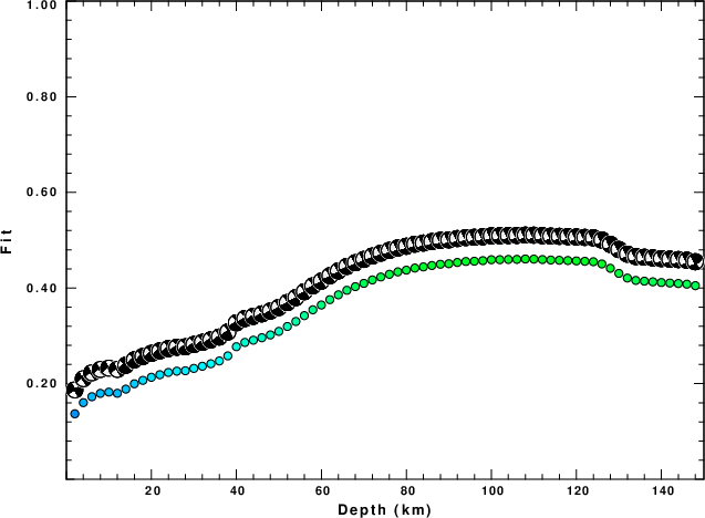
The best fit as a function of depth is given in the following figure:
|
|
Figure 2. Depth sensitivity for waveform mechanism
|
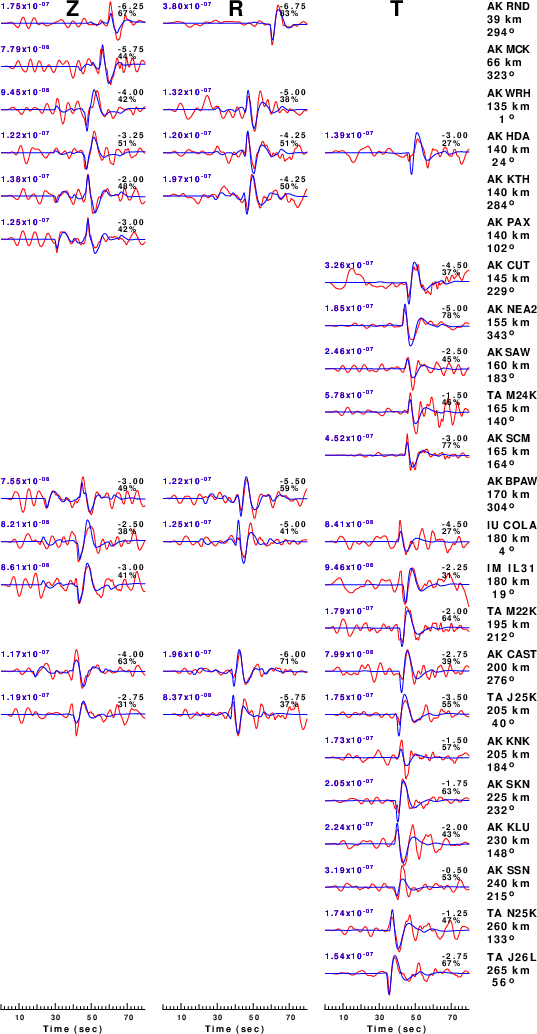
The comparison of the observed and predicted waveforms is given in the next figure. The red traces are the observed and the blue are the predicted.
Each observed-predicted component is plotted to the same scale and peak amplitudes are indicated by the numbers to the left of each trace. A pair of numbers is given in black at the right of each predicted traces. The upper number it the time shift required for maximum correlation between the observed and predicted traces. This time shift is required because the synthetics are not computed at exactly the same distance as the observed, the velocity model used in the predictions may not be perfect and the epicentral parameters may be be off.
A positive time shift indicates that the prediction is too fast and should be delayed to match the observed trace (shift to the right in this figure). A negative value indicates that the prediction is too slow. The lower number gives the percentage of variance reduction to characterize the individual goodness of fit (100% indicates a perfect fit).
The bandpass filter used in the processing and for the display was
cut o DIST/3.3 -50 o DIST/3.3 +30
rtr
taper w 0.1
hp c 0.03 n 3
lp c 0.10 n 3
|
|
Figure 3. Waveform comparison for selected depth. Red: observed; Blue - predicted. The time shift with respect to the model prediction is indicated. The percent of fit is also indicated. The time scale is relative to the first trace sample.
|
|
|
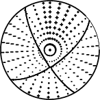
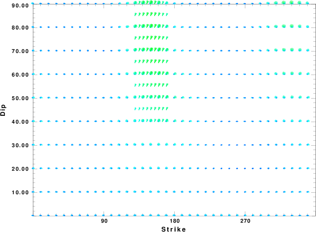
Focal mechanism sensitivity at the preferred depth. The red color indicates a very good fit to the waveforms.
Each solution is plotted as a vector at a given value of strike and dip with the angle of the vector representing the rake angle, measured, with respect to the upward vertical (N) in the figure.
|
A check on the assumed source location is possible by looking at the time shifts between the observed and predicted traces. The time shifts for waveform matching arise for several reasons:
- The origin time and epicentral distance are incorrect
- The velocity model used for the inversion is incorrect
- The velocity model used to define the P-arrival time is not the
same as the velocity model used for the waveform inversion
(assuming that the initial trace alignment is based on the
P arrival time)
Assuming only a mislocation, the time shifts are fit to a functional form:
Time_shift = A + B cos Azimuth + C Sin Azimuth
The time shifts for this inversion lead to the next figure:
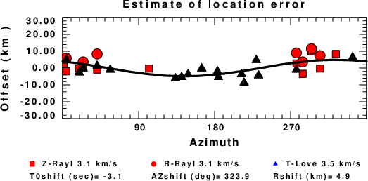
The derived shift in origin time and epicentral coordinates are given at the bottom of the figure.
Velocity Model
The WUS.model used for the waveform synthetic seismograms and for the surface wave eigenfunctions and dispersion is as follows
(The format is in the model96 format of Computer Programs in Seismology).
MODEL.01
Model after     8 iterations
ISOTROPIC
KGS
FLAT EARTH
1-D
CONSTANT VELOCITY
LINE08
LINE09
LINE10
LINE11
      H(KM)   VP(KM/S)   VS(KM/S) RHO(GM/CC)         QP         QS       ETAP       ETAS      FREFP      FREFS
     1.9000     3.4065     2.0089     2.2150  0.302E-02  0.679E-02   0.00       0.00       1.00       1.00
     6.1000     5.5445     3.2953     2.6089  0.349E-02  0.784E-02   0.00       0.00       1.00       1.00
    13.0000     6.2708     3.7396     2.7812  0.212E-02  0.476E-02   0.00       0.00       1.00       1.00
    19.0000     6.4075     3.7680     2.8223  0.111E-02  0.249E-02   0.00       0.00       1.00       1.00
     0.0000     7.9000     4.6200     3.2760  0.164E-10  0.370E-10   0.00       0.00       1.00       1.00
Last Changed Thu Apr 25 11:38:23 PM CDT 2024