Location
SLU Location
Because the moment tensor solution wanted a depth near 50 km and the ANSS location was 28 km, P and S first arrival times were read and the program elocate was run. The output of the program is elocate.txt. When started with a depth of 10 km, the solution converged to a depth of 39 km, but the first motion plot was incompatible with the moment tensor nodal planes. When the program was started with a depth of 100, it converged to a depth of 54 km with a marginally smaller RMS error in time. The P-wave first motion data for this latter solution was in agreement with the
moment tensor solution.
Location ANSS
The ANSS event ID is ak0182plgsrf and the event page is at
https://earthquake.usgs.gov/earthquakes/eventpage/ak0182plgsrf/executive.
2018/02/28 01:27:47 62.349 -148.729 39.5 4.3 Alaska
Focal Mechanism
 USGS/SLU Moment Tensor Solution
 ENS  2018/02/28 01:27:47:0  62.35 -148.73  39.5 4.3 Alaska

 Stations used:
   AK.CAST AK.DHY AK.GHO AK.KLU AK.KNK AK.KTH AK.MLY AK.NEA2
   AK.RC01 AK.RND AK.SAW AK.SCM AK.SSN AK.TRF AT.PMR TA.M22K
   TA.M24K TA.POKR

 Filtering commands used:
   cut o DIST/3.3 -30 o DIST/3.3 +40
   rtr
   taper w 0.1
   hp c 0.03 n 3
   lp c 0.08 n 3

 Best Fitting Double Couple
  Mo = 3.43e+22 dyne-cm
  Mw = 4.29
  Z  = 52 km
  Plane   Strike  Dip  Rake
   NP1      290    55   -55
   NP2       59    48   -129
  Principal Axes:
   Axis    Value   Plunge  Azimuth
    T   3.43e+22      4     356
    N   0.00e+00     28      88
    P  -3.43e+22     62     259

 Moment Tensor: (dyne-cm)
    Component   Value
       Mxx     3.37e+22
       Mxy    -3.86e+21
       Mxz     5.17e+21
       Myy    -7.27e+21
       Myz     1.39e+22
       Mzz    -2.64e+22


                     #### T #######
                 ########   ###########
              ############################
             ##############################
           ##################################
          #######------#######################
         ##--------------------###############-
        ---------------------------##########---
        ------------------------------#######---
       ----------------------------------###-----
       -------------   --------------------------
       ------------- P -------------------##-----
       -------------   ------------------#####---
        -------------------------------########-
        -----------------------------##########-
         --------------------------############
          ---------------------###############
           ##--------------##################
             ##############################
              ############################
                 ######################
                     ##############


 Global CMT Convention Moment Tensor:
      R          T          P
 -2.64e+22   5.17e+21  -1.39e+22
  5.17e+21   3.37e+22   3.86e+21
 -1.39e+22   3.86e+21  -7.27e+21


Details of the solution is found at

http://www.eas.slu.edu/eqc/eqc_mt/MECH.NA/20180228012747/index.html
|
Preferred Solution
The preferred solution from an analysis of the surface-wave spectral amplitude radiation pattern, waveform inversion or first motion observations is
      STK = 290
      DIP = 55
     RAKE = -55
       MW = 4.29
       HS = 52.0
The NDK file is 20180228012747.ndk
The waveform inversion is preferred.
Moment Tensor Comparison
The following compares this source inversion to those provided by others. The purpose is to look for major differences and also to note slight differences that might be inherent to the processing procedure. For completeness the USGS/SLU solution is repeated from above.
| SLU |
SLUFM |
 USGS/SLU Moment Tensor Solution
 ENS  2018/02/28 01:27:47:0  62.35 -148.73  39.5 4.3 Alaska

 Stations used:
   AK.CAST AK.DHY AK.GHO AK.KLU AK.KNK AK.KTH AK.MLY AK.NEA2
   AK.RC01 AK.RND AK.SAW AK.SCM AK.SSN AK.TRF AT.PMR TA.M22K
   TA.M24K TA.POKR

 Filtering commands used:
   cut o DIST/3.3 -30 o DIST/3.3 +40
   rtr
   taper w 0.1
   hp c 0.03 n 3
   lp c 0.08 n 3

 Best Fitting Double Couple
  Mo = 3.43e+22 dyne-cm
  Mw = 4.29
  Z  = 52 km
  Plane   Strike  Dip  Rake
   NP1      290    55   -55
   NP2       59    48   -129
  Principal Axes:
   Axis    Value   Plunge  Azimuth
    T   3.43e+22      4     356
    N   0.00e+00     28      88
    P  -3.43e+22     62     259

 Moment Tensor: (dyne-cm)
    Component   Value
       Mxx     3.37e+22
       Mxy    -3.86e+21
       Mxz     5.17e+21
       Myy    -7.27e+21
       Myz     1.39e+22
       Mzz    -2.64e+22


                     #### T #######
                 ########   ###########
              ############################
             ##############################
           ##################################
          #######------#######################
         ##--------------------###############-
        ---------------------------##########---
        ------------------------------#######---
       ----------------------------------###-----
       -------------   --------------------------
       ------------- P -------------------##-----
       -------------   ------------------#####---
        -------------------------------########-
        -----------------------------##########-
         --------------------------############
          ---------------------###############
           ##--------------##################
             ##############################
              ############################
                 ######################
                     ##############


 Global CMT Convention Moment Tensor:
      R          T          P
 -2.64e+22   5.17e+21  -1.39e+22
  5.17e+21   3.37e+22   3.86e+21
 -1.39e+22   3.86e+21  -7.27e+21


Details of the solution is found at

http://www.eas.slu.edu/eqc/eqc_mt/MECH.NA/20180228012747/index.html
|
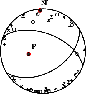
First motions and takeoff angles from an elocate run.
|
Magnitudes
Given the availability of digital waveforms for determination of the moment tensor, this section documents the added processing leading to mLg, if appropriate to the region, and ML by application of the respective IASPEI formulae. As a research study, the linear distance term of the IASPEI formula
for ML is adjusted to remove a linear distance trend in residuals to give a regionally defined ML. The defined ML uses horizontal component recordings, but the same procedure is applied to the vertical components since there may be some interest in vertical component ground motions. Residual plots versus distance may indicate interesting features of ground motion scaling in some distance ranges. A residual plot of the regionalized magnitude is given as a function of distance and azimuth, since data sets may transcend different wave propagation provinces.
ML Magnitude
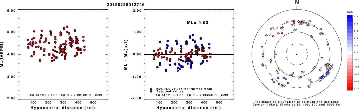
Left: ML computed using the IASPEI formula for Horizontal components. Center: ML residuals computed using a modified IASPEI formula that accounts for path specific attenuation; the values used for the trimmed mean are indicated. The ML relation used for each figure is given at the bottom of each plot.
Right: Residuals from new relation as a function of distance and azimuth.
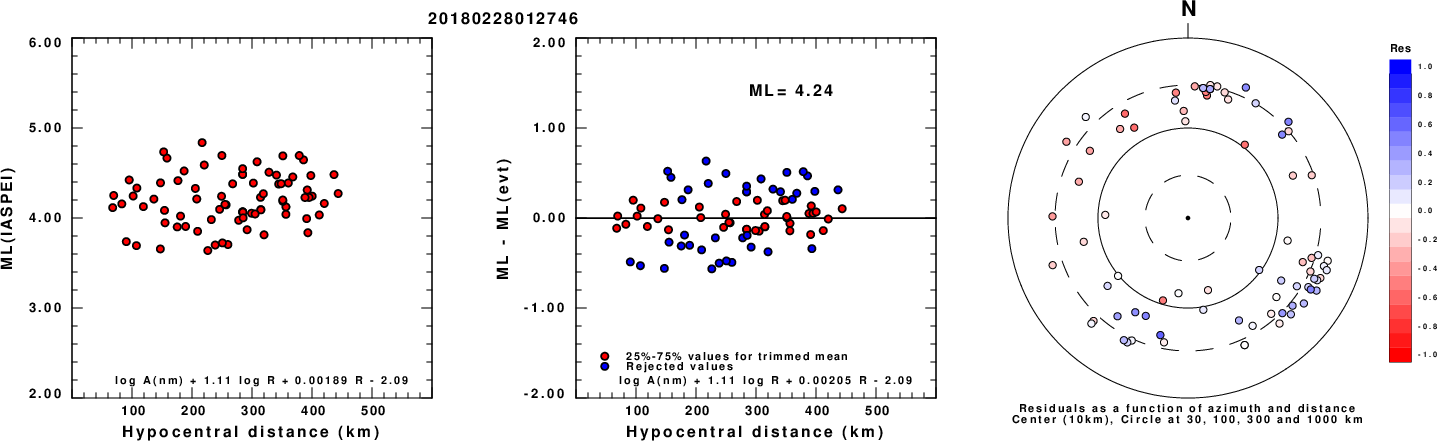
Left: ML computed using the IASPEI formula for Vertical components (research). Center: ML residuals computed using a modified IASPEI formula that accounts for path specific attenuation; the values used for the trimmed mean are indicated. The ML relation used for each figure is given at the bottom of each plot.
Right: Residuals from new relation as a function of distance and azimuth.
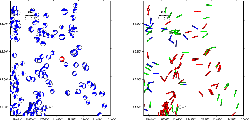
Context
The left panel of the next figure presents the focal mechanism for this earthquake (red) in the context of other nearby events (blue) in the SLU Moment Tensor Catalog. The right panel shows the inferred direction of maximum compressive stress and the type of faulting (green is strike-slip, red is normal, blue is thrust; oblique is shown by a combination of colors). Thus context plot is useful for assessing the appropriateness of the moment tensor of this event.
Waveform Inversion using wvfgrd96
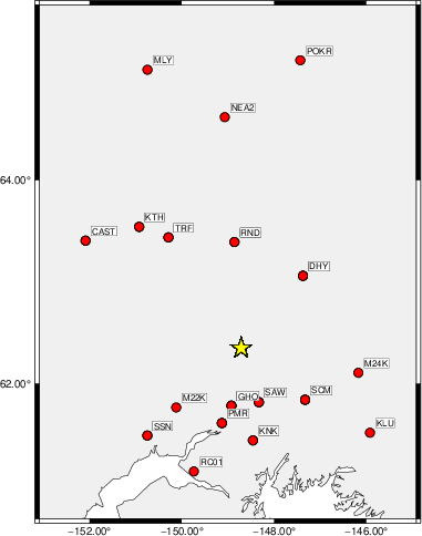
The focal mechanism was determined using broadband seismic waveforms. The location of the event (star) and the
stations used for (red) the waveform inversion are shown in the next figure.
|
|
Location of broadband stations used for waveform inversion
|
The program wvfgrd96 was used with good traces observed at short distance to determine the focal mechanism, depth and seismic moment. This technique requires a high quality signal and well determined velocity model for the Green's functions. To the extent that these are the quality data, this type of mechanism should be preferred over the radiation pattern technique which requires the separate step of defining the pressure and tension quadrants and the correct strike.
The observed and predicted traces are filtered using the following gsac commands:
cut o DIST/3.3 -30 o DIST/3.3 +40
rtr
taper w 0.1
hp c 0.03 n 3
lp c 0.08 n 3
The results of this grid search are as follow:
           DEPTH  STK   DIP  RAKE   MW    FIT
WVFGRD96    2.0    65    50    55   3.55 0.2865
WVFGRD96    4.0   240    70    50   3.64 0.3186
WVFGRD96    6.0    35    55   -40   3.69 0.3523
WVFGRD96    8.0    30    50   -45   3.77 0.3676
WVFGRD96   10.0    35    60   -40   3.78 0.3712
WVFGRD96   12.0   335    50    50   3.84 0.3874
WVFGRD96   14.0   330    55    45   3.85 0.3980
WVFGRD96   16.0   330    55    45   3.88 0.4036
WVFGRD96   18.0   145    60    35   3.88 0.4145
WVFGRD96   20.0   145    60    35   3.91 0.4278
WVFGRD96   22.0   145    60    35   3.93 0.4389
WVFGRD96   24.0   140    70    30   3.94 0.4497
WVFGRD96   26.0   140    70    25   3.96 0.4621
WVFGRD96   28.0   140    75    25   3.98 0.4728
WVFGRD96   30.0   310    60   -15   4.01 0.5008
WVFGRD96   32.0   310    60   -20   4.03 0.5275
WVFGRD96   34.0   305    60   -25   4.05 0.5531
WVFGRD96   36.0   305    60   -25   4.07 0.5775
WVFGRD96   38.0   300    60   -30   4.10 0.5999
WVFGRD96   40.0   295    50   -40   4.18 0.6234
WVFGRD96   42.0   295    50   -45   4.21 0.6363
WVFGRD96   44.0   295    55   -45   4.22 0.6472
WVFGRD96   46.0   295    55   -45   4.24 0.6604
WVFGRD96   48.0   290    55   -50   4.26 0.6699
WVFGRD96   50.0   290    55   -55   4.28 0.6771
WVFGRD96   52.0   290    55   -55   4.29 0.6810
WVFGRD96   54.0   290    55   -55   4.29 0.6807
WVFGRD96   56.0   290    55   -55   4.30 0.6763
WVFGRD96   58.0   295    60   -45   4.30 0.6712
WVFGRD96   60.0   295    60   -45   4.30 0.6643
WVFGRD96   62.0   290    60   -50   4.31 0.6566
WVFGRD96   64.0   290    60   -50   4.31 0.6486
WVFGRD96   66.0   295    65   -45   4.31 0.6392
WVFGRD96   68.0   295    65   -45   4.31 0.6320
WVFGRD96   70.0   295    65   -40   4.31 0.6260
WVFGRD96   72.0   295    65   -40   4.31 0.6194
WVFGRD96   74.0   295    65   -40   4.31 0.6124
WVFGRD96   76.0   295    70   -40   4.32 0.6079
WVFGRD96   78.0   295    70   -40   4.32 0.6031
WVFGRD96   80.0   295    70   -40   4.32 0.5977
WVFGRD96   82.0   295    70   -40   4.32 0.5916
WVFGRD96   84.0   295    70   -40   4.32 0.5857
WVFGRD96   86.0   295    70   -40   4.32 0.5796
WVFGRD96   88.0   295    70   -40   4.32 0.5735
WVFGRD96   90.0   295    75   -40   4.33 0.5678
WVFGRD96   92.0   295    75   -40   4.33 0.5632
WVFGRD96   94.0   295    75   -40   4.34 0.5580
WVFGRD96   96.0   295    75   -40   4.34 0.5530
WVFGRD96   98.0   300    75   -30   4.33 0.5488
The best solution is
WVFGRD96 52.0 290 55 -55 4.29 0.6810
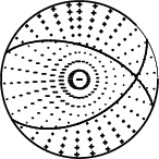
The mechanism corresponding to the best fit is
|
|
Figure 1. Waveform inversion focal mechanism
|
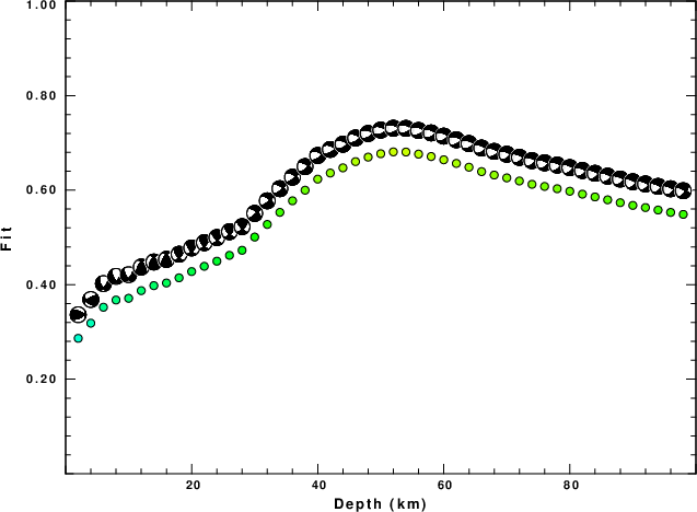
The best fit as a function of depth is given in the following figure:
|
|
Figure 2. Depth sensitivity for waveform mechanism
|
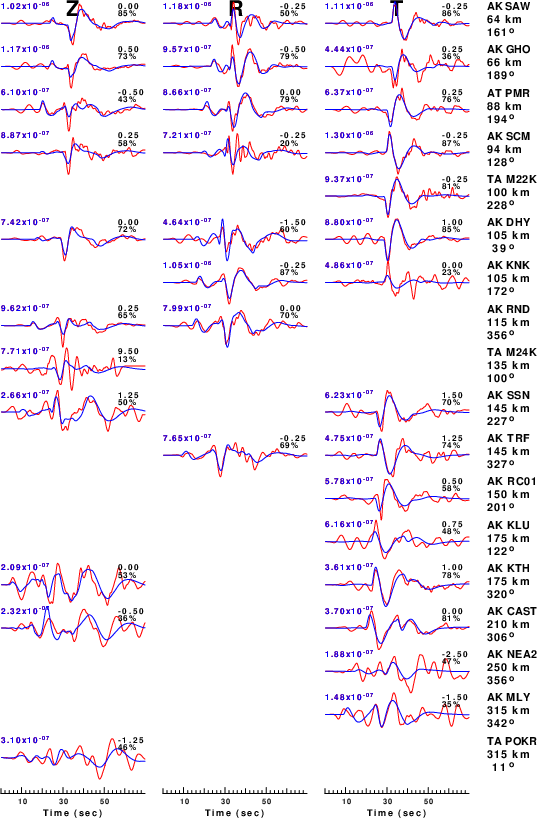
The comparison of the observed and predicted waveforms is given in the next figure. The red traces are the observed and the blue are the predicted.
Each observed-predicted component is plotted to the same scale and peak amplitudes are indicated by the numbers to the left of each trace. A pair of numbers is given in black at the right of each predicted traces. The upper number it the time shift required for maximum correlation between the observed and predicted traces. This time shift is required because the synthetics are not computed at exactly the same distance as the observed, the velocity model used in the predictions may not be perfect and the epicentral parameters may be be off.
A positive time shift indicates that the prediction is too fast and should be delayed to match the observed trace (shift to the right in this figure). A negative value indicates that the prediction is too slow. The lower number gives the percentage of variance reduction to characterize the individual goodness of fit (100% indicates a perfect fit).
The bandpass filter used in the processing and for the display was
cut o DIST/3.3 -30 o DIST/3.3 +40
rtr
taper w 0.1
hp c 0.03 n 3
lp c 0.08 n 3
|
|
Figure 3. Waveform comparison for selected depth. Red: observed; Blue - predicted. The time shift with respect to the model prediction is indicated. The percent of fit is also indicated. The time scale is relative to the first trace sample.
|
|
|
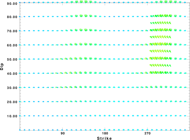
Focal mechanism sensitivity at the preferred depth. The red color indicates a very good fit to the waveforms.
Each solution is plotted as a vector at a given value of strike and dip with the angle of the vector representing the rake angle, measured, with respect to the upward vertical (N) in the figure.
|
A check on the assumed source location is possible by looking at the time shifts between the observed and predicted traces. The time shifts for waveform matching arise for several reasons:
- The origin time and epicentral distance are incorrect
- The velocity model used for the inversion is incorrect
- The velocity model used to define the P-arrival time is not the
same as the velocity model used for the waveform inversion
(assuming that the initial trace alignment is based on the
P arrival time)
Assuming only a mislocation, the time shifts are fit to a functional form:
Time_shift = A + B cos Azimuth + C Sin Azimuth
The time shifts for this inversion lead to the next figure:
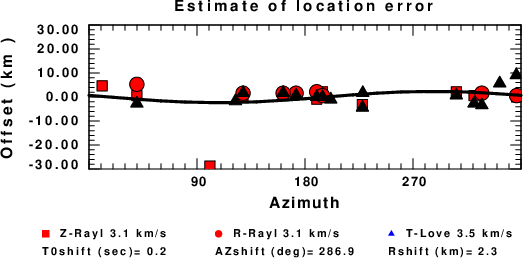
The derived shift in origin time and epicentral coordinates are given at the bottom of the figure.
Velocity Model
The WUS.model used for the waveform synthetic seismograms and for the surface wave eigenfunctions and dispersion is as follows
(The format is in the model96 format of Computer Programs in Seismology).
MODEL.01
Model after     8 iterations
ISOTROPIC
KGS
FLAT EARTH
1-D
CONSTANT VELOCITY
LINE08
LINE09
LINE10
LINE11
      H(KM)   VP(KM/S)   VS(KM/S) RHO(GM/CC)         QP         QS       ETAP       ETAS      FREFP      FREFS
     1.9000     3.4065     2.0089     2.2150  0.302E-02  0.679E-02   0.00       0.00       1.00       1.00
     6.1000     5.5445     3.2953     2.6089  0.349E-02  0.784E-02   0.00       0.00       1.00       1.00
    13.0000     6.2708     3.7396     2.7812  0.212E-02  0.476E-02   0.00       0.00       1.00       1.00
    19.0000     6.4075     3.7680     2.8223  0.111E-02  0.249E-02   0.00       0.00       1.00       1.00
     0.0000     7.9000     4.6200     3.2760  0.164E-10  0.370E-10   0.00       0.00       1.00       1.00
Last Changed Thu Apr 25 09:28:29 PM CDT 2024