Location
Location ANSS
The ANSS event ID is ak0177q3cz5d and the event page is at
https://earthquake.usgs.gov/earthquakes/eventpage/ak0177q3cz5d/executive.
2017/06/17 15:24:10 62.465 -149.089 39.4 3.7 Alaska
Focal Mechanism
 USGS/SLU Moment Tensor Solution
 ENS  2017/06/17 15:24:10:0  62.47 -149.09  39.4 3.7 Alaska

 Stations used:
   AK.BWN AK.CUT AK.DHY AK.GLI AK.KLU AK.KNK AK.MCK AK.RC01
   AK.RND AK.SAW AK.SCM AT.PMR TA.K20K TA.M22K TA.M24K

 Filtering commands used:
   cut o DIST/3.5 -30 o DIST/3.5 +50
   rtr
   taper w 0.1
   hp c 0.04 n 3
   lp c 0.12 n 3

 Best Fitting Double Couple
  Mo = 4.79e+21 dyne-cm
  Mw = 3.72
  Z  = 60 km
  Plane   Strike  Dip  Rake
   NP1      305    75   -40
   NP2       47    52   -161
  Principal Axes:
   Axis    Value   Plunge  Azimuth
    T   4.79e+21     15       1
    N   0.00e+00     48     108
    P  -4.79e+21     38     259

 Moment Tensor: (dyne-cm)
    Component   Value
       Mxx     4.36e+21
       Mxy    -4.89e+20
       Mxz     1.64e+21
       Myy    -2.82e+21
       Myz     2.31e+21
       Mzz    -1.54e+21


                     ######   #####
                 ########## T #########
              #############   ############
             ##############################
           ################################--
          -------##########################---
         -------------#####################----
        -----------------##################-----
        --------------------##############------
       ------------------------###########-------
       --------------------------########--------
       -------   ------------------#####---------
       ------- P --------------------------------
        ------   --------------------##---------
        ---------------------------######-------
         ------------------------##########----
          ---------------------#############--
           ----------------##################
             ----------####################
              ############################
                 ######################
                     ##############


 Global CMT Convention Moment Tensor:
      R          T          P
 -1.54e+21   1.64e+21  -2.31e+21
  1.64e+21   4.36e+21   4.89e+20
 -2.31e+21   4.89e+20  -2.82e+21


Details of the solution is found at

http://www.eas.slu.edu/eqc/eqc_mt/MECH.NA/20170617152410/index.html
|
Preferred Solution
The preferred solution from an analysis of the surface-wave spectral amplitude radiation pattern, waveform inversion or first motion observations is
      STK = 305
      DIP = 75
     RAKE = -40
       MW = 3.72
       HS = 60.0
The NDK file is 20170617152410.ndk
The waveform inversion is preferred.
Magnitudes
Given the availability of digital waveforms for determination of the moment tensor, this section documents the added processing leading to mLg, if appropriate to the region, and ML by application of the respective IASPEI formulae. As a research study, the linear distance term of the IASPEI formula
for ML is adjusted to remove a linear distance trend in residuals to give a regionally defined ML. The defined ML uses horizontal component recordings, but the same procedure is applied to the vertical components since there may be some interest in vertical component ground motions. Residual plots versus distance may indicate interesting features of ground motion scaling in some distance ranges. A residual plot of the regionalized magnitude is given as a function of distance and azimuth, since data sets may transcend different wave propagation provinces.
ML Magnitude
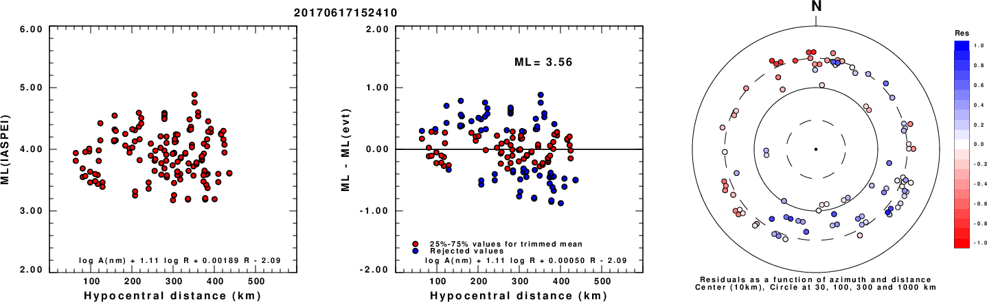
Left: ML computed using the IASPEI formula for Horizontal components. Center: ML residuals computed using a modified IASPEI formula that accounts for path specific attenuation; the values used for the trimmed mean are indicated. The ML relation used for each figure is given at the bottom of each plot.
Right: Residuals from new relation as a function of distance and azimuth.
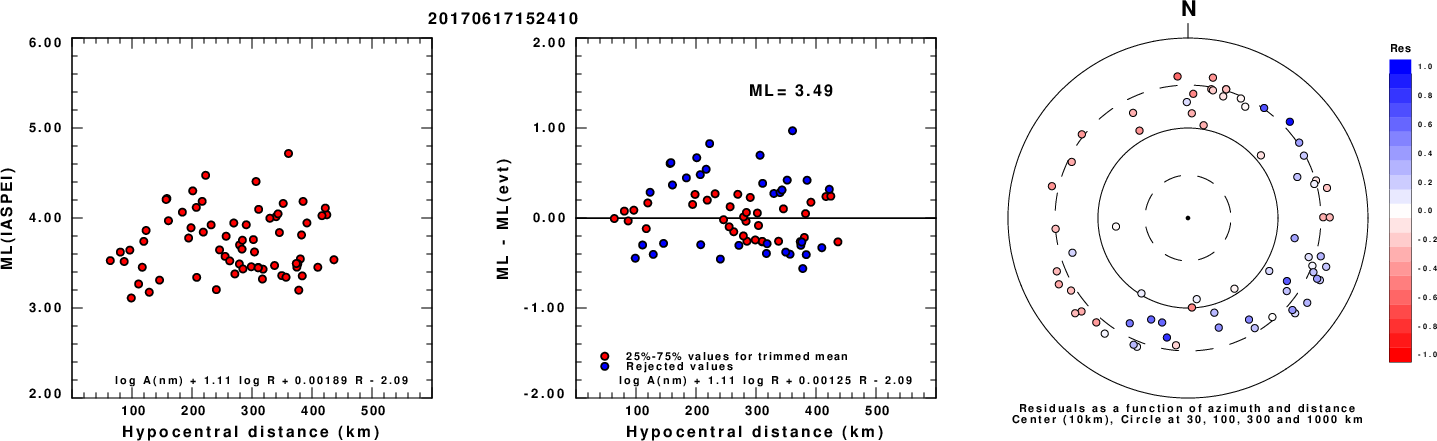
Left: ML computed using the IASPEI formula for Vertical components (research). Center: ML residuals computed using a modified IASPEI formula that accounts for path specific attenuation; the values used for the trimmed mean are indicated. The ML relation used for each figure is given at the bottom of each plot.
Right: Residuals from new relation as a function of distance and azimuth.
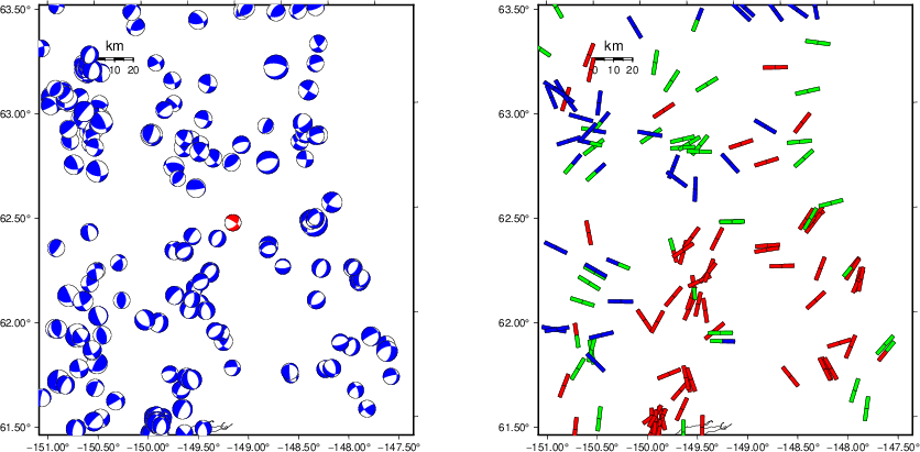
Context
The left panel of the next figure presents the focal mechanism for this earthquake (red) in the context of other nearby events (blue) in the SLU Moment Tensor Catalog. The right panel shows the inferred direction of maximum compressive stress and the type of faulting (green is strike-slip, red is normal, blue is thrust; oblique is shown by a combination of colors). Thus context plot is useful for assessing the appropriateness of the moment tensor of this event.
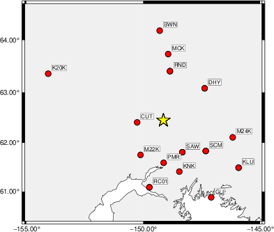
Waveform Inversion using wvfgrd96
The focal mechanism was determined using broadband seismic waveforms. The location of the event (star) and the
stations used for (red) the waveform inversion are shown in the next figure.
|
|
Location of broadband stations used for waveform inversion
|
The program wvfgrd96 was used with good traces observed at short distance to determine the focal mechanism, depth and seismic moment. This technique requires a high quality signal and well determined velocity model for the Green's functions. To the extent that these are the quality data, this type of mechanism should be preferred over the radiation pattern technique which requires the separate step of defining the pressure and tension quadrants and the correct strike.
The observed and predicted traces are filtered using the following gsac commands:
cut o DIST/3.5 -30 o DIST/3.5 +50
rtr
taper w 0.1
hp c 0.04 n 3
lp c 0.12 n 3
The results of this grid search are as follow:
           DEPTH  STK   DIP  RAKE   MW    FIT
WVFGRD96    1.0   220    80    -5   2.64 0.1362
WVFGRD96    2.0   220    90    -5   2.79 0.1785
WVFGRD96    3.0    50    80    40   2.91 0.1961
WVFGRD96    4.0    50    80    40   2.96 0.2134
WVFGRD96    5.0    30    40   -30   3.04 0.2340
WVFGRD96    6.0    30    40   -30   3.07 0.2515
WVFGRD96    7.0    35    45   -25   3.10 0.2628
WVFGRD96    8.0    30    40   -30   3.17 0.2685
WVFGRD96    9.0    35    40   -25   3.20 0.2715
WVFGRD96   10.0    35    40   -25   3.22 0.2719
WVFGRD96   11.0    35    45   -20   3.24 0.2697
WVFGRD96   12.0    35    45   -20   3.26 0.2662
WVFGRD96   13.0    45    50    10   3.26 0.2620
WVFGRD96   14.0    45    50    10   3.28 0.2586
WVFGRD96   15.0    45    50    10   3.30 0.2539
WVFGRD96   16.0    45    50    10   3.31 0.2482
WVFGRD96   17.0    45    50    10   3.33 0.2405
WVFGRD96   18.0   125    75   -35   3.32 0.2426
WVFGRD96   19.0   125    75   -35   3.34 0.2501
WVFGRD96   20.0   130    80   -35   3.36 0.2596
WVFGRD96   21.0   130    80   -30   3.37 0.2703
WVFGRD96   22.0   315    75    40   3.41 0.2854
WVFGRD96   23.0   315    75    40   3.43 0.3000
WVFGRD96   24.0   315    75    40   3.45 0.3138
WVFGRD96   25.0   315    75    40   3.46 0.3265
WVFGRD96   26.0   315    75    35   3.46 0.3370
WVFGRD96   27.0   320    75    40   3.48 0.3477
WVFGRD96   28.0   315    80    35   3.47 0.3564
WVFGRD96   29.0   315    55    10   3.48 0.3657
WVFGRD96   30.0   315    55    10   3.49 0.3767
WVFGRD96   31.0   310    60    -5   3.48 0.3854
WVFGRD96   32.0   310    55    -5   3.49 0.3949
WVFGRD96   33.0   310    55    -5   3.50 0.4030
WVFGRD96   34.0   310    55   -10   3.51 0.4098
WVFGRD96   35.0   310    55   -10   3.51 0.4138
WVFGRD96   36.0   310    55   -10   3.52 0.4169
WVFGRD96   37.0   310    60   -15   3.52 0.4192
WVFGRD96   38.0   310    60   -15   3.54 0.4234
WVFGRD96   39.0   310    60   -15   3.55 0.4285
WVFGRD96   40.0   305    55   -25   3.61 0.4264
WVFGRD96   41.0   305    50   -20   3.63 0.4294
WVFGRD96   42.0   305    55   -25   3.64 0.4312
WVFGRD96   43.0   305    55   -25   3.65 0.4311
WVFGRD96   44.0   305    55   -25   3.66 0.4305
WVFGRD96   45.0   305    65   -35   3.67 0.4310
WVFGRD96   46.0   305    65   -35   3.67 0.4334
WVFGRD96   47.0   305    65   -35   3.68 0.4353
WVFGRD96   48.0   305    65   -35   3.69 0.4376
WVFGRD96   49.0   305    65   -35   3.69 0.4413
WVFGRD96   50.0   305    65   -35   3.70 0.4443
WVFGRD96   51.0   305    70   -40   3.70 0.4465
WVFGRD96   52.0   305    70   -40   3.71 0.4482
WVFGRD96   53.0   305    70   -40   3.71 0.4505
WVFGRD96   54.0   305    70   -40   3.71 0.4531
WVFGRD96   55.0   305    70   -40   3.71 0.4549
WVFGRD96   56.0   305    70   -40   3.72 0.4546
WVFGRD96   57.0   305    70   -40   3.72 0.4564
WVFGRD96   58.0   305    70   -40   3.72 0.4555
WVFGRD96   59.0   305    75   -40   3.72 0.4555
WVFGRD96   60.0   305    75   -40   3.72 0.4576
WVFGRD96   61.0   305    75   -40   3.72 0.4571
WVFGRD96   62.0   305    75   -40   3.72 0.4554
WVFGRD96   63.0   305    75   -40   3.72 0.4566
WVFGRD96   64.0   305    75   -40   3.72 0.4555
WVFGRD96   65.0   305    75   -40   3.72 0.4563
WVFGRD96   66.0   305    75   -40   3.72 0.4557
WVFGRD96   67.0   305    75   -40   3.72 0.4525
WVFGRD96   68.0   305    75   -40   3.73 0.4553
WVFGRD96   69.0   305    75   -40   3.73 0.4522
WVFGRD96   70.0   305    75   -40   3.73 0.4525
WVFGRD96   71.0   305    75   -40   3.73 0.4514
WVFGRD96   72.0   305    80   -45   3.74 0.4513
WVFGRD96   73.0   305    80   -40   3.73 0.4493
WVFGRD96   74.0   305    80   -45   3.74 0.4488
WVFGRD96   75.0   305    80   -40   3.73 0.4484
WVFGRD96   76.0   305    80   -40   3.73 0.4457
WVFGRD96   77.0   305    80   -40   3.73 0.4462
WVFGRD96   78.0   295    70   -55   3.75 0.4446
WVFGRD96   79.0   305    80   -40   3.73 0.4420
WVFGRD96   80.0   295    70   -55   3.75 0.4428
WVFGRD96   81.0   295    70   -55   3.75 0.4393
WVFGRD96   82.0   295    70   -55   3.75 0.4403
WVFGRD96   83.0   295    70   -55   3.75 0.4365
WVFGRD96   84.0   300    75   -50   3.75 0.4362
WVFGRD96   85.0   300    75   -50   3.75 0.4353
WVFGRD96   86.0   300    75   -50   3.75 0.4339
WVFGRD96   87.0   300    75   -50   3.75 0.4337
WVFGRD96   88.0   295    70   -55   3.75 0.4318
WVFGRD96   89.0   295    70   -55   3.76 0.4317
WVFGRD96   90.0   295    70   -55   3.76 0.4288
WVFGRD96   91.0   295    70   -55   3.76 0.4297
WVFGRD96   92.0   295    70   -55   3.76 0.4276
WVFGRD96   93.0   295    70   -55   3.76 0.4272
WVFGRD96   94.0   295    70   -55   3.76 0.4268
WVFGRD96   95.0   295    70   -55   3.76 0.4244
WVFGRD96   96.0   295    70   -55   3.76 0.4255
WVFGRD96   97.0   295    70   -55   3.76 0.4227
WVFGRD96   98.0   295    70   -55   3.76 0.4235
WVFGRD96   99.0   295    70   -55   3.76 0.4214
The best solution is
WVFGRD96 60.0 305 75 -40 3.72 0.4576
The mechanism corresponding to the best fit is
|
|
Figure 1. Waveform inversion focal mechanism
|
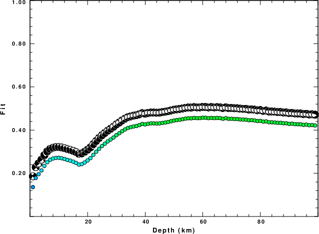
The best fit as a function of depth is given in the following figure:
|
|
Figure 2. Depth sensitivity for waveform mechanism
|
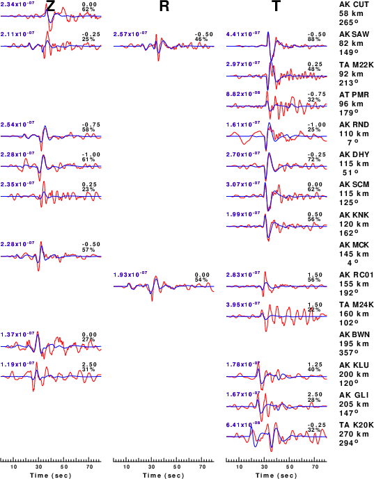
The comparison of the observed and predicted waveforms is given in the next figure. The red traces are the observed and the blue are the predicted.
Each observed-predicted component is plotted to the same scale and peak amplitudes are indicated by the numbers to the left of each trace. A pair of numbers is given in black at the right of each predicted traces. The upper number it the time shift required for maximum correlation between the observed and predicted traces. This time shift is required because the synthetics are not computed at exactly the same distance as the observed, the velocity model used in the predictions may not be perfect and the epicentral parameters may be be off.
A positive time shift indicates that the prediction is too fast and should be delayed to match the observed trace (shift to the right in this figure). A negative value indicates that the prediction is too slow. The lower number gives the percentage of variance reduction to characterize the individual goodness of fit (100% indicates a perfect fit).
The bandpass filter used in the processing and for the display was
cut o DIST/3.5 -30 o DIST/3.5 +50
rtr
taper w 0.1
hp c 0.04 n 3
lp c 0.12 n 3
|
|
Figure 3. Waveform comparison for selected depth. Red: observed; Blue - predicted. The time shift with respect to the model prediction is indicated. The percent of fit is also indicated. The time scale is relative to the first trace sample.
|
|
|
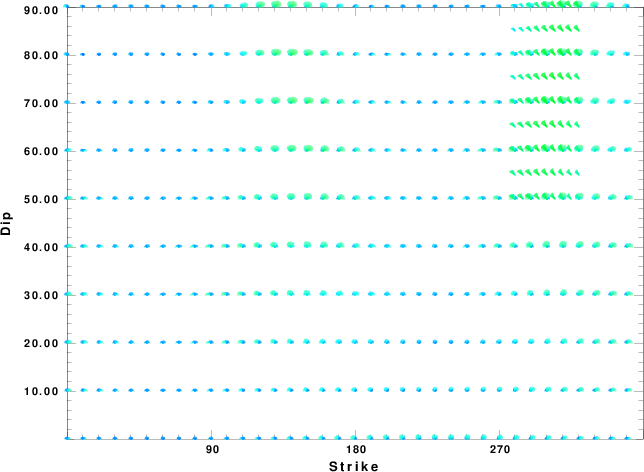
Focal mechanism sensitivity at the preferred depth. The red color indicates a very good fit to the waveforms.
Each solution is plotted as a vector at a given value of strike and dip with the angle of the vector representing the rake angle, measured, with respect to the upward vertical (N) in the figure.
|
A check on the assumed source location is possible by looking at the time shifts between the observed and predicted traces. The time shifts for waveform matching arise for several reasons:
- The origin time and epicentral distance are incorrect
- The velocity model used for the inversion is incorrect
- The velocity model used to define the P-arrival time is not the
same as the velocity model used for the waveform inversion
(assuming that the initial trace alignment is based on the
P arrival time)
Assuming only a mislocation, the time shifts are fit to a functional form:
Time_shift = A + B cos Azimuth + C Sin Azimuth
The time shifts for this inversion lead to the next figure:
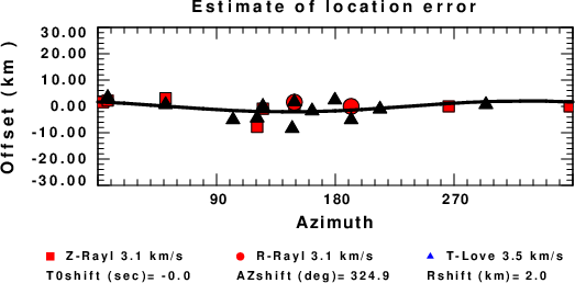
The derived shift in origin time and epicentral coordinates are given at the bottom of the figure.
Velocity Model
The WUS.model used for the waveform synthetic seismograms and for the surface wave eigenfunctions and dispersion is as follows
(The format is in the model96 format of Computer Programs in Seismology).
MODEL.01
Model after     8 iterations
ISOTROPIC
KGS
FLAT EARTH
1-D
CONSTANT VELOCITY
LINE08
LINE09
LINE10
LINE11
      H(KM)   VP(KM/S)   VS(KM/S) RHO(GM/CC)         QP         QS       ETAP       ETAS      FREFP      FREFS
     1.9000     3.4065     2.0089     2.2150  0.302E-02  0.679E-02   0.00       0.00       1.00       1.00
     6.1000     5.5445     3.2953     2.6089  0.349E-02  0.784E-02   0.00       0.00       1.00       1.00
    13.0000     6.2708     3.7396     2.7812  0.212E-02  0.476E-02   0.00       0.00       1.00       1.00
    19.0000     6.4075     3.7680     2.8223  0.111E-02  0.249E-02   0.00       0.00       1.00       1.00
     0.0000     7.9000     4.6200     3.2760  0.164E-10  0.370E-10   0.00       0.00       1.00       1.00
Last Changed Sat Apr 27 02:15:37 PM CDT 2024