Location
Location ANSS
The ANSS event ID is ak0172sx1gks and the event page is at
https://earthquake.usgs.gov/earthquakes/eventpage/ak0172sx1gks/executive.
2017/03/02 02:11:30 59.578 -152.655 78.0 5.6 Alaska
Focal Mechanism
 USGS/SLU Moment Tensor Solution
 ENS  2017/03/02 02:11:30:0  59.58 -152.65  78.0 5.6 Alaska

 Stations used:
   AK.BRLK AK.CAPN AK.CAST AK.CNP AK.CUT AK.FIRE AK.GHO AK.HOM
   AK.PWL AK.RC01 AK.SKN AK.SSN AK.SWD AT.OHAK AT.PMR AT.SVW2
   AV.ILSW II.KDAK TA.M22K TA.N19K TA.O19K TA.O22K TA.P18K
   TA.Q19K

 Filtering commands used:
   cut o DIST/3.3 -50 o DIST/3.3 +50
   rtr
   taper w 0.1
   hp c 0.03 n 3
   lp c 0.10 n 3

 Best Fitting Double Couple
  Mo = 2.66e+24 dyne-cm
  Mw = 5.55
  Z  = 90 km
  Plane   Strike  Dip  Rake
   NP1      302    66   141
   NP2       50    55    30
  Principal Axes:
   Axis    Value   Plunge  Azimuth
    T   2.66e+24     44     262
    N   0.00e+00     45      95
    P  -2.66e+24      7     358

 Moment Tensor: (dyne-cm)
    Component   Value
       Mxx    -2.59e+24
       Mxy     2.88e+23
       Mxz    -5.01e+23
       Myy     1.34e+24
       Myz    -1.30e+24
       Mzz     1.25e+24


                     ----- P ------
                 ---------   ----------
              ----------------------------
             ------------------------------
           ---------------------------------#
          ##########------------------------##
         ################-------------------###
        #####################--------------#####
        ########################----------######
       ############################------########
       ########   ###################---#########
       ######## T ###############################
       ########   ####################---########
        ############################------######
        ##########################----------####
         #######################-------------##
          ###################----------------#
           ##############--------------------
             ------------------------------
              ----------------------------
                 ----------------------
                     --------------


 Global CMT Convention Moment Tensor:
      R          T          P
  1.25e+24  -5.01e+23   1.30e+24
 -5.01e+23  -2.59e+24  -2.88e+23
  1.30e+24  -2.88e+23   1.34e+24


Details of the solution is found at

http://www.eas.slu.edu/eqc/eqc_mt/MECH.NA/20170302021130/index.html
|
Preferred Solution
The preferred solution from an analysis of the surface-wave spectral amplitude radiation pattern, waveform inversion or first motion observations is
      STK = 50
      DIP = 55
     RAKE = 30
       MW = 5.55
       HS = 90.0
The NDK file is 20170302021130.ndk
The waveform inversion is preferred.
Moment Tensor Comparison
The following compares this source inversion to those provided by others. The purpose is to look for major differences and also to note slight differences that might be inherent to the processing procedure. For completeness the USGS/SLU solution is repeated from above.
| SLU |
USGSMT |
USGSMWR |
 USGS/SLU Moment Tensor Solution
 ENS  2017/03/02 02:11:30:0  59.58 -152.65  78.0 5.6 Alaska

 Stations used:
   AK.BRLK AK.CAPN AK.CAST AK.CNP AK.CUT AK.FIRE AK.GHO AK.HOM
   AK.PWL AK.RC01 AK.SKN AK.SSN AK.SWD AT.OHAK AT.PMR AT.SVW2
   AV.ILSW II.KDAK TA.M22K TA.N19K TA.O19K TA.O22K TA.P18K
   TA.Q19K

 Filtering commands used:
   cut o DIST/3.3 -50 o DIST/3.3 +50
   rtr
   taper w 0.1
   hp c 0.03 n 3
   lp c 0.10 n 3

 Best Fitting Double Couple
  Mo = 2.66e+24 dyne-cm
  Mw = 5.55
  Z  = 90 km
  Plane   Strike  Dip  Rake
   NP1      302    66   141
   NP2       50    55    30
  Principal Axes:
   Axis    Value   Plunge  Azimuth
    T   2.66e+24     44     262
    N   0.00e+00     45      95
    P  -2.66e+24      7     358

 Moment Tensor: (dyne-cm)
    Component   Value
       Mxx    -2.59e+24
       Mxy     2.88e+23
       Mxz    -5.01e+23
       Myy     1.34e+24
       Myz    -1.30e+24
       Mzz     1.25e+24


                     ----- P ------
                 ---------   ----------
              ----------------------------
             ------------------------------
           ---------------------------------#
          ##########------------------------##
         ################-------------------###
        #####################--------------#####
        ########################----------######
       ############################------########
       ########   ###################---#########
       ######## T ###############################
       ########   ####################---########
        ############################------######
        ##########################----------####
         #######################-------------##
          ###################----------------#
           ##############--------------------
             ------------------------------
              ----------------------------
                 ----------------------
                     --------------


 Global CMT Convention Moment Tensor:
      R          T          P
  1.25e+24  -5.01e+23   1.30e+24
 -5.01e+23  -2.59e+24  -2.88e+23
  1.30e+24  -2.88e+23   1.34e+24


Details of the solution is found at

http://www.eas.slu.edu/eqc/eqc_mt/MECH.NA/20170302021130/index.html
|
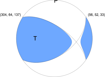
Nody-wave Moment Tensor (Mwb)
Moment	2.921e+17 N-m
Magnitude	5.6 Mwb
Depth	76.0 km
Percent DC	94 %
Half Duration	–
Catalog	US
Data Source	US3
Contributor	US3
Nodal Planes
Plane	Strike	Dip	Rake
NP1	304	64	137
NP2	56	52	33
Principal Axes
Axis	Value	Plunge	Azimuth
T	2.968e+17 N-m	48	264
N	-0.096e+17 N-m	41	99
P	-2.871e+17 N-m	7	3
|
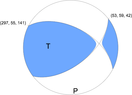
Regional Moment Tensor (Mwr)
Moment	2.663e+17 N-m
Magnitude	5.6 Mwr
Depth	80.0 km
Percent DC	98 %
Half Duration	–
Catalog	US
Data Source	US3
Contributor	US3
Nodal Planes
Plane	Strike	Dip	Rake
NP1	297	55	141
NP2	53	59	42
Principal Axes
Axis	Value	Plunge	Azimuth
T	2.676e+17 N-m	51	267
N	-0.028e+17 N-m	39	82
P	-2.649e+17 N-m	2	174
|
Magnitudes
Given the availability of digital waveforms for determination of the moment tensor, this section documents the added processing leading to mLg, if appropriate to the region, and ML by application of the respective IASPEI formulae. As a research study, the linear distance term of the IASPEI formula
for ML is adjusted to remove a linear distance trend in residuals to give a regionally defined ML. The defined ML uses horizontal component recordings, but the same procedure is applied to the vertical components since there may be some interest in vertical component ground motions. Residual plots versus distance may indicate interesting features of ground motion scaling in some distance ranges. A residual plot of the regionalized magnitude is given as a function of distance and azimuth, since data sets may transcend different wave propagation provinces.
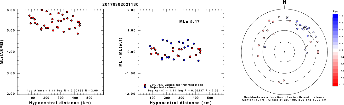
ML Magnitude
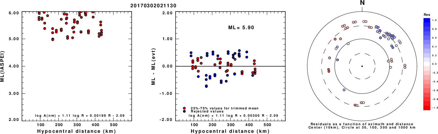
Left: ML computed using the IASPEI formula for Horizontal components. Center: ML residuals computed using a modified IASPEI formula that accounts for path specific attenuation; the values used for the trimmed mean are indicated. The ML relation used for each figure is given at the bottom of each plot.
Right: Residuals from new relation as a function of distance and azimuth.
Left: ML computed using the IASPEI formula for Vertical components (research). Center: ML residuals computed using a modified IASPEI formula that accounts for path specific attenuation; the values used for the trimmed mean are indicated. The ML relation used for each figure is given at the bottom of each plot.
Right: Residuals from new relation as a function of distance and azimuth.
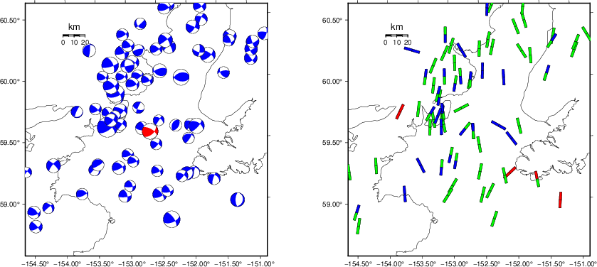
Context
The left panel of the next figure presents the focal mechanism for this earthquake (red) in the context of other nearby events (blue) in the SLU Moment Tensor Catalog. The right panel shows the inferred direction of maximum compressive stress and the type of faulting (green is strike-slip, red is normal, blue is thrust; oblique is shown by a combination of colors). Thus context plot is useful for assessing the appropriateness of the moment tensor of this event.
Waveform Inversion using wvfgrd96
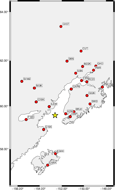
The focal mechanism was determined using broadband seismic waveforms. The location of the event (star) and the
stations used for (red) the waveform inversion are shown in the next figure.
|
|
Location of broadband stations used for waveform inversion
|
The program wvfgrd96 was used with good traces observed at short distance to determine the focal mechanism, depth and seismic moment. This technique requires a high quality signal and well determined velocity model for the Green's functions. To the extent that these are the quality data, this type of mechanism should be preferred over the radiation pattern technique which requires the separate step of defining the pressure and tension quadrants and the correct strike.
The observed and predicted traces are filtered using the following gsac commands:
cut o DIST/3.3 -50 o DIST/3.3 +50
rtr
taper w 0.1
hp c 0.03 n 3
lp c 0.10 n 3
The results of this grid search are as follow:
           DEPTH  STK   DIP  RAKE   MW    FIT
WVFGRD96    2.0    80    40   -85   4.68 0.1511
WVFGRD96    4.0   300    70    30   4.69 0.1717
WVFGRD96    6.0   290    55   -25   4.73 0.1921
WVFGRD96    8.0   290    55   -30   4.82 0.2145
WVFGRD96   10.0   300    65    25   4.87 0.2287
WVFGRD96   12.0   300    65    25   4.90 0.2368
WVFGRD96   14.0   300    65    25   4.92 0.2335
WVFGRD96   16.0    35    65    25   4.94 0.2294
WVFGRD96   18.0    25    55    -5   4.98 0.2317
WVFGRD96   20.0    25    60    -5   5.02 0.2469
WVFGRD96   22.0    25    55    -5   5.05 0.2605
WVFGRD96   24.0    25    55    -5   5.07 0.2713
WVFGRD96   26.0    25    55    -5   5.10 0.2776
WVFGRD96   28.0    25    55    -5   5.11 0.2795
WVFGRD96   30.0    30    55     0   5.12 0.2809
WVFGRD96   32.0    30    60     5   5.14 0.2820
WVFGRD96   34.0    30    60     5   5.15 0.2809
WVFGRD96   36.0    35    65    10   5.16 0.2807
WVFGRD96   38.0    35    65    10   5.19 0.2868
WVFGRD96   40.0    35    55    10   5.27 0.2992
WVFGRD96   42.0    35    60    10   5.28 0.3022
WVFGRD96   44.0    35    60    15   5.31 0.3057
WVFGRD96   46.0    40    60    20   5.33 0.3090
WVFGRD96   48.0    40    60    20   5.35 0.3126
WVFGRD96   50.0    40    60    20   5.36 0.3158
WVFGRD96   52.0    40    60    20   5.37 0.3192
WVFGRD96   54.0    40    60    25   5.39 0.3237
WVFGRD96   56.0    45    60    30   5.41 0.3309
WVFGRD96   58.0    45    60    30   5.42 0.3387
WVFGRD96   60.0    45    60    30   5.43 0.3491
WVFGRD96   62.0    45    60    30   5.44 0.3597
WVFGRD96   64.0    50    55    30   5.46 0.3706
WVFGRD96   66.0    50    55    30   5.47 0.3818
WVFGRD96   68.0    50    55    30   5.48 0.3920
WVFGRD96   70.0    50    55    30   5.49 0.4020
WVFGRD96   72.0    50    55    30   5.50 0.4104
WVFGRD96   74.0    50    55    30   5.51 0.4182
WVFGRD96   76.0    50    60    30   5.52 0.4252
WVFGRD96   78.0    50    60    30   5.53 0.4299
WVFGRD96   80.0    50    60    30   5.53 0.4339
WVFGRD96   82.0    50    55    30   5.53 0.4364
WVFGRD96   84.0    50    55    30   5.54 0.4385
WVFGRD96   86.0    50    55    30   5.54 0.4407
WVFGRD96   88.0    50    55    30   5.55 0.4410
WVFGRD96   90.0    50    55    30   5.55 0.4415
WVFGRD96   92.0    50    55    30   5.55 0.4403
WVFGRD96   94.0    50    55    30   5.55 0.4382
WVFGRD96   96.0    50    55    30   5.56 0.4361
WVFGRD96   98.0    50    55    30   5.56 0.4339
The best solution is
WVFGRD96 90.0 50 55 30 5.55 0.4415
The mechanism corresponding to the best fit is
|
|
Figure 1. Waveform inversion focal mechanism
|
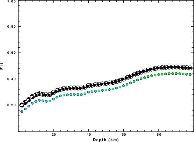
The best fit as a function of depth is given in the following figure:
|
|
Figure 2. Depth sensitivity for waveform mechanism
|
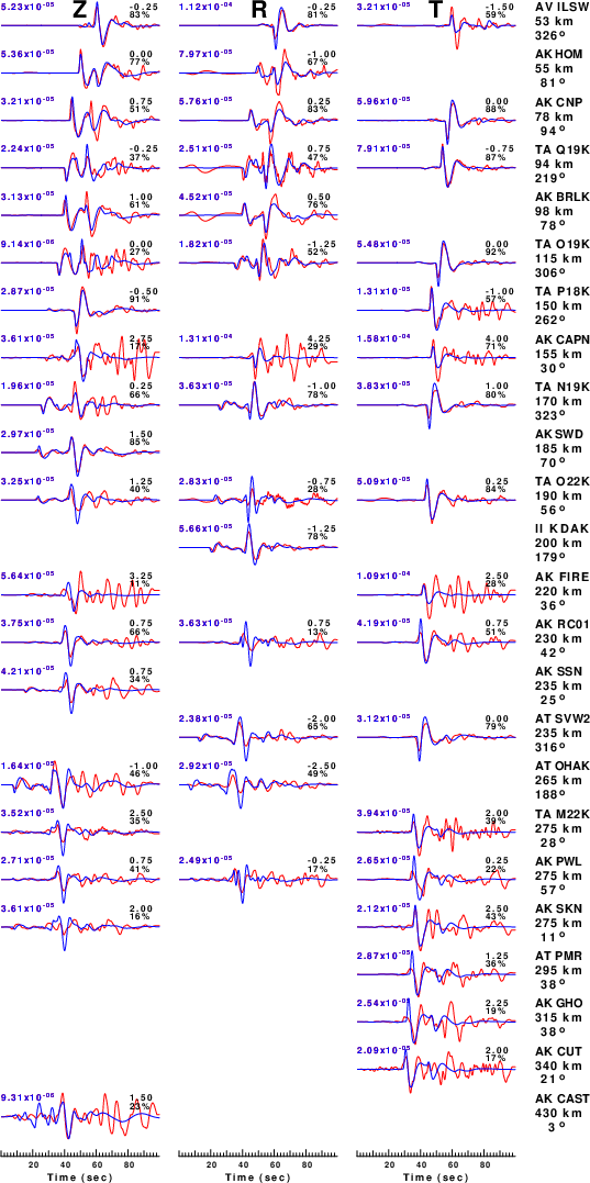
The comparison of the observed and predicted waveforms is given in the next figure. The red traces are the observed and the blue are the predicted.
Each observed-predicted component is plotted to the same scale and peak amplitudes are indicated by the numbers to the left of each trace. A pair of numbers is given in black at the right of each predicted traces. The upper number it the time shift required for maximum correlation between the observed and predicted traces. This time shift is required because the synthetics are not computed at exactly the same distance as the observed, the velocity model used in the predictions may not be perfect and the epicentral parameters may be be off.
A positive time shift indicates that the prediction is too fast and should be delayed to match the observed trace (shift to the right in this figure). A negative value indicates that the prediction is too slow. The lower number gives the percentage of variance reduction to characterize the individual goodness of fit (100% indicates a perfect fit).
The bandpass filter used in the processing and for the display was
cut o DIST/3.3 -50 o DIST/3.3 +50
rtr
taper w 0.1
hp c 0.03 n 3
lp c 0.10 n 3
|
|
Figure 3. Waveform comparison for selected depth. Red: observed; Blue - predicted. The time shift with respect to the model prediction is indicated. The percent of fit is also indicated. The time scale is relative to the first trace sample.
|
|
|
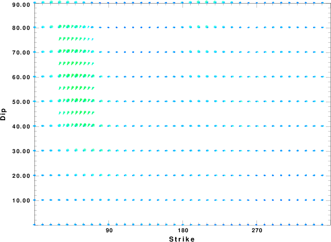
Focal mechanism sensitivity at the preferred depth. The red color indicates a very good fit to the waveforms.
Each solution is plotted as a vector at a given value of strike and dip with the angle of the vector representing the rake angle, measured, with respect to the upward vertical (N) in the figure.
|
A check on the assumed source location is possible by looking at the time shifts between the observed and predicted traces. The time shifts for waveform matching arise for several reasons:
- The origin time and epicentral distance are incorrect
- The velocity model used for the inversion is incorrect
- The velocity model used to define the P-arrival time is not the
same as the velocity model used for the waveform inversion
(assuming that the initial trace alignment is based on the
P arrival time)
Assuming only a mislocation, the time shifts are fit to a functional form:
Time_shift = A + B cos Azimuth + C Sin Azimuth
The time shifts for this inversion lead to the next figure:
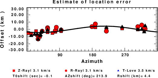
The derived shift in origin time and epicentral coordinates are given at the bottom of the figure.
Velocity Model
The WUS.model used for the waveform synthetic seismograms and for the surface wave eigenfunctions and dispersion is as follows
(The format is in the model96 format of Computer Programs in Seismology).
MODEL.01
Model after     8 iterations
ISOTROPIC
KGS
FLAT EARTH
1-D
CONSTANT VELOCITY
LINE08
LINE09
LINE10
LINE11
      H(KM)   VP(KM/S)   VS(KM/S) RHO(GM/CC)         QP         QS       ETAP       ETAS      FREFP      FREFS
     1.9000     3.4065     2.0089     2.2150  0.302E-02  0.679E-02   0.00       0.00       1.00       1.00
     6.1000     5.5445     3.2953     2.6089  0.349E-02  0.784E-02   0.00       0.00       1.00       1.00
    13.0000     6.2708     3.7396     2.7812  0.212E-02  0.476E-02   0.00       0.00       1.00       1.00
    19.0000     6.4075     3.7680     2.8223  0.111E-02  0.249E-02   0.00       0.00       1.00       1.00
     0.0000     7.9000     4.6200     3.2760  0.164E-10  0.370E-10   0.00       0.00       1.00       1.00
Last Changed Sat Apr 27 11:42:29 AM CDT 2024