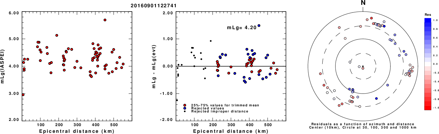
Left: mLg computed using the IASPEI formula. Center: mLg residuals versus epicentral distance ; the values used for the trimmed mean magnitude estimate are indicated. Right: residuals as a function of distance and azimuth.
The ANSS event ID is ak016b9dz3vp and the event page is at https://earthquake.usgs.gov/earthquakes/eventpage/ak016b9dz3vp/executive.
2016/09/01 12:27:41 61.299 -152.165 131.7 4.5 Alaska
 USGS/SLU Moment Tensor Solution
 ENS  2016/09/01 12:27:41:0  61.30 -152.16 131.7 4.5 Alaska

 Stations used:
   AK.BRSE AK.CHUM AK.SLK AK.WAT1 AK.WAT6 AK.WAT7 AV.AUJA
   AV.NCT AV.RDDF AV.RDSO AV.RDWB AV.RED AV.SPNN TA.K24K
   TA.L20K TA.M23K TA.N16K TA.N20K TA.O16K TA.O17K TA.O18K
   TA.O20K TA.P16K TA.Q16K TA.Q20K XV.FAPT XV.FPAP XV.FTGH

 Filtering commands used:
   cut a -20 a 100
   rtr
   taper w 0.1
   hp c 0.02 n 3
   lp c 0.10 n 3

 Best Fitting Double Couple
  Mo = 5.96e+22 dyne-cm
  Mw = 4.45
  Z  = 128 km
  Plane   Strike  Dip  Rake
   NP1      307    51   124
   NP2       80    50    55
  Principal Axes:
   Axis    Value   Plunge  Azimuth
    T   5.96e+22     64     283
    N   0.00e+00     26     104
    P  -5.96e+22      1      14

 Moment Tensor: (dyne-cm)
    Component   Value
       Mxx    -5.56e+22
       Mxy    -1.64e+22
       Mxz     4.53e+21
       Myy     7.50e+21
       Myz    -2.31e+22
       Mzz     4.81e+22


                     ----------- P
                 ---------------   ----
              ----------------------------
             ------------------------------
           ###############-------------------
          ####################----------------
         ########################--------------
        ############################------------
        #############################-----------
       #############   ################---------#
       ############# T #################-------##
       #############   ###################----###
       ####################################-#####
        -#################################-#####
        ---############################-----####
         -----#####################---------###
          -----------#######-----------------#
           ----------------------------------
             ------------------------------
              ----------------------------
                 ----------------------
                     --------------


 Global CMT Convention Moment Tensor:
      R          T          P
  4.81e+22   4.53e+21   2.31e+22
  4.53e+21  -5.56e+22   1.64e+22
  2.31e+22   1.64e+22   7.50e+21


Details of the solution is found at

http://www.eas.slu.edu/eqc/eqc_mt/MECH.NA/20160901122741/index.html
|
      STK = 80
      DIP = 50
     RAKE = 55
       MW = 4.45
       HS = 128.0
The NDK file is 20160901122741.ndk The waveform inversion is preferred.
Given the availability of digital waveforms for determination of the moment tensor, this section documents the added processing leading to mLg, if appropriate to the region, and ML by application of the respective IASPEI formulae. As a research study, the linear distance term of the IASPEI formula for ML is adjusted to remove a linear distance trend in residuals to give a regionally defined ML. The defined ML uses horizontal component recordings, but the same procedure is applied to the vertical components since there may be some interest in vertical component ground motions. Residual plots versus distance may indicate interesting features of ground motion scaling in some distance ranges. A residual plot of the regionalized magnitude is given as a function of distance and azimuth, since data sets may transcend different wave propagation provinces.
Left: mLg computed using the IASPEI formula. Center: mLg residuals versus epicentral distance ; the values used for the trimmed mean magnitude estimate are indicated.
Right: residuals as a function of distance and azimuth.
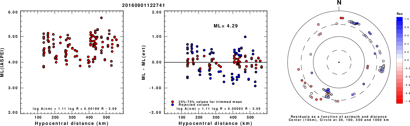
Left: ML computed using the IASPEI formula for Horizontal components. Center: ML residuals computed using a modified IASPEI formula that accounts for path specific attenuation; the values used for the trimmed mean are indicated. The ML relation used for each figure is given at the bottom of each plot.
Right: Residuals from new relation as a function of distance and azimuth.
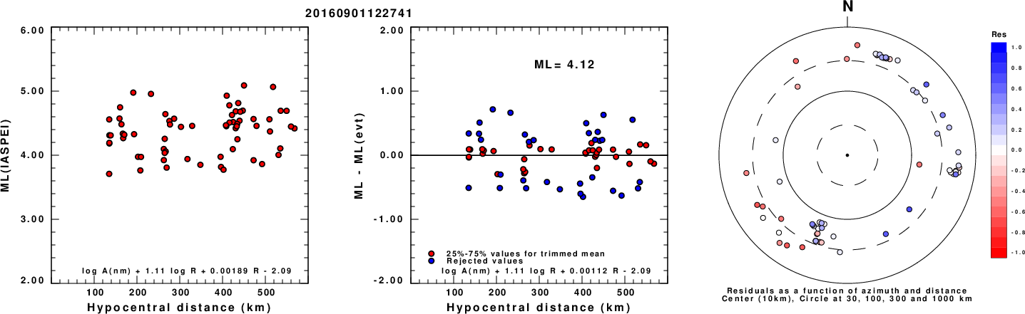
Left: ML computed using the IASPEI formula for Vertical components (research). Center: ML residuals computed using a modified IASPEI formula that accounts for path specific attenuation; the values used for the trimmed mean are indicated. The ML relation used for each figure is given at the bottom of each plot.
Right: Residuals from new relation as a function of distance and azimuth.
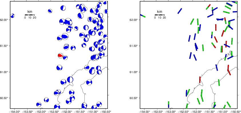 |
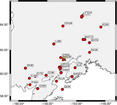
The focal mechanism was determined using broadband seismic waveforms. The location of the event (star) and the stations used for (red) the waveform inversion are shown in the next figure.
|
|
|
The program wvfgrd96 was used with good traces observed at short distance to determine the focal mechanism, depth and seismic moment. This technique requires a high quality signal and well determined velocity model for the Green's functions. To the extent that these are the quality data, this type of mechanism should be preferred over the radiation pattern technique which requires the separate step of defining the pressure and tension quadrants and the correct strike.
The observed and predicted traces are filtered using the following gsac commands:
cut a -20 a 100
rtr
taper w 0.1
hp c 0.02 n 3
lp c 0.10 n 3
The results of this grid search are as follow:
           DEPTH  STK   DIP  RAKE   MW    FIT
WVFGRD96    2.0    95    55   -85   3.59 0.1614
WVFGRD96    4.0   335    30   -15   3.67 0.1614
WVFGRD96    6.0   335    35   -10   3.70 0.1913
WVFGRD96    8.0   340    35     0   3.78 0.1974
WVFGRD96   10.0    -5    35    30   3.82 0.2035
WVFGRD96   12.0   195    40   -35   3.82 0.2149
WVFGRD96   14.0   190    40   -35   3.86 0.2315
WVFGRD96   16.0   190    40   -35   3.90 0.2399
WVFGRD96   18.0   195    40   -25   3.92 0.2405
WVFGRD96   20.0   195    35   -25   3.93 0.2365
WVFGRD96   22.0   205    35   -10   3.95 0.2288
WVFGRD96   24.0   210    35     0   3.97 0.2197
WVFGRD96   26.0   215    35    10   3.98 0.2098
WVFGRD96   28.0   200    35   -15   4.03 0.2015
WVFGRD96   30.0   205    35    -5   4.04 0.1954
WVFGRD96   32.0   210    35     0   4.05 0.1901
WVFGRD96   34.0   210    35     0   4.06 0.1878
WVFGRD96   36.0   250    80    15   4.11 0.1876
WVFGRD96   38.0    65    50    50   4.06 0.1946
WVFGRD96   40.0   155    70   -30   4.20 0.2152
WVFGRD96   42.0   155    70   -30   4.24 0.2217
WVFGRD96   44.0   155    70   -30   4.26 0.2255
WVFGRD96   46.0   150    65   -40   4.26 0.2304
WVFGRD96   48.0   145    60   -45   4.27 0.2335
WVFGRD96   50.0   145    60   -40   4.29 0.2344
WVFGRD96   52.0    90    65    70   4.26 0.2379
WVFGRD96   54.0   280    25   105   4.27 0.2528
WVFGRD96   56.0    90    65    70   4.29 0.2760
WVFGRD96   58.0   245    35    55   4.31 0.2949
WVFGRD96   60.0   245    35    55   4.32 0.3140
WVFGRD96   62.0    90    65    70   4.33 0.3344
WVFGRD96   64.0    85    65    65   4.35 0.3516
WVFGRD96   66.0    85    65    65   4.36 0.3686
WVFGRD96   68.0    85    65    65   4.36 0.3836
WVFGRD96   70.0    85    65    65   4.37 0.3973
WVFGRD96   72.0    85    65    65   4.38 0.4092
WVFGRD96   74.0    85    65    65   4.38 0.4202
WVFGRD96   76.0    80    65    60   4.40 0.4310
WVFGRD96   78.0    80    65    60   4.40 0.4402
WVFGRD96   80.0    80    65    60   4.41 0.4491
WVFGRD96   82.0    80    65    60   4.41 0.4564
WVFGRD96   84.0    80    60    60   4.41 0.4636
WVFGRD96   86.0    80    60    60   4.41 0.4706
WVFGRD96   88.0    80    60    60   4.41 0.4772
WVFGRD96   90.0    80    60    60   4.42 0.4829
WVFGRD96   92.0    80    60    55   4.43 0.4876
WVFGRD96   94.0    80    60    55   4.43 0.4918
WVFGRD96   96.0    80    55    60   4.42 0.4957
WVFGRD96   98.0    80    55    60   4.42 0.5000
WVFGRD96  100.0    80    55    60   4.42 0.5032
WVFGRD96  102.0    80    55    60   4.43 0.5057
WVFGRD96  104.0    80    55    60   4.43 0.5086
WVFGRD96  106.0    80    55    60   4.43 0.5116
WVFGRD96  108.0    80    55    60   4.43 0.5146
WVFGRD96  110.0    80    55    55   4.44 0.5165
WVFGRD96  112.0    75    55    55   4.44 0.5174
WVFGRD96  114.0    75    55    55   4.45 0.5188
WVFGRD96  116.0    75    55    55   4.45 0.5202
WVFGRD96  118.0    75    55    55   4.45 0.5219
WVFGRD96  120.0    75    55    55   4.45 0.5234
WVFGRD96  122.0    80    50    55   4.45 0.5234
WVFGRD96  124.0    80    50    55   4.45 0.5237
WVFGRD96  126.0    80    50    55   4.45 0.5251
WVFGRD96  128.0    80    50    55   4.45 0.5253
WVFGRD96  130.0    80    50    55   4.45 0.5243
WVFGRD96  132.0    75    50    50   4.46 0.5248
WVFGRD96  134.0    75    50    50   4.46 0.5241
WVFGRD96  136.0    75    50    50   4.46 0.5238
WVFGRD96  138.0    75    50    50   4.47 0.5232
WVFGRD96  140.0    75    50    50   4.47 0.5217
WVFGRD96  142.0    75    50    50   4.47 0.5213
WVFGRD96  144.0    75    50    50   4.47 0.5194
WVFGRD96  146.0    75    50    50   4.47 0.5184
WVFGRD96  148.0    75    50    50   4.47 0.5170
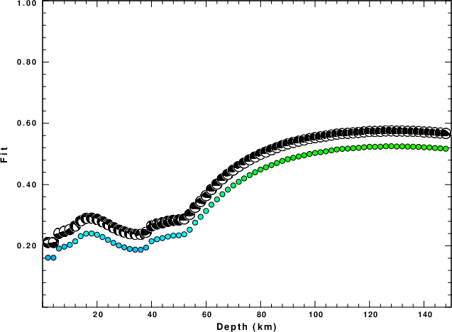
The best solution is
WVFGRD96 128.0 80 50 55 4.45 0.5253
The mechanism corresponding to the best fit is
|
|
|
The best fit as a function of depth is given in the following figure:
|
|
|
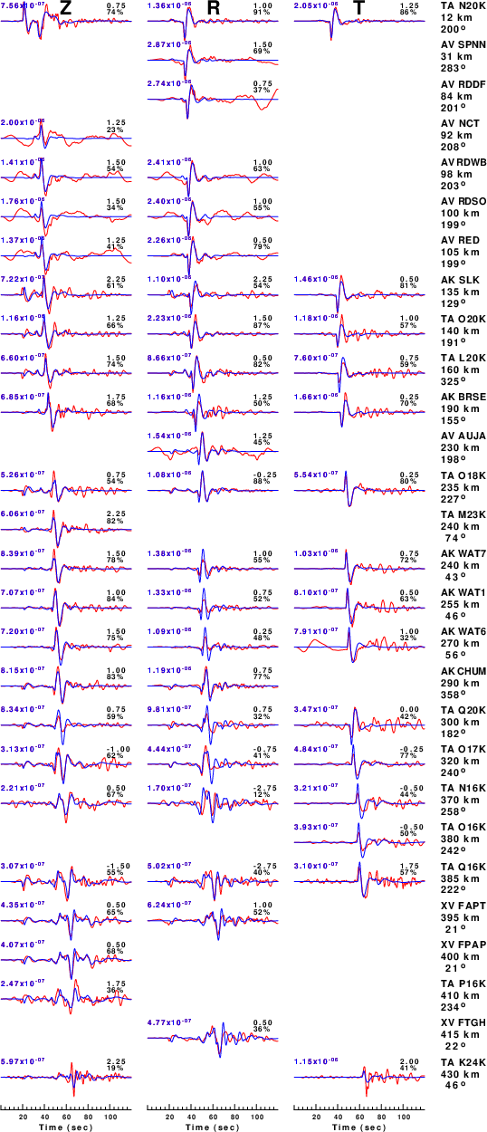
The comparison of the observed and predicted waveforms is given in the next figure. The red traces are the observed and the blue are the predicted. Each observed-predicted component is plotted to the same scale and peak amplitudes are indicated by the numbers to the left of each trace. A pair of numbers is given in black at the right of each predicted traces. The upper number it the time shift required for maximum correlation between the observed and predicted traces. This time shift is required because the synthetics are not computed at exactly the same distance as the observed, the velocity model used in the predictions may not be perfect and the epicentral parameters may be be off. A positive time shift indicates that the prediction is too fast and should be delayed to match the observed trace (shift to the right in this figure). A negative value indicates that the prediction is too slow. The lower number gives the percentage of variance reduction to characterize the individual goodness of fit (100% indicates a perfect fit).
The bandpass filter used in the processing and for the display was
cut a -20 a 100
rtr
taper w 0.1
hp c 0.02 n 3
lp c 0.10 n 3
|
| Figure 3. Waveform comparison for selected depth. Red: observed; Blue - predicted. The time shift with respect to the model prediction is indicated. The percent of fit is also indicated. The time scale is relative to the first trace sample. |
|
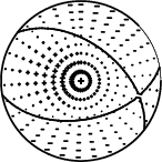
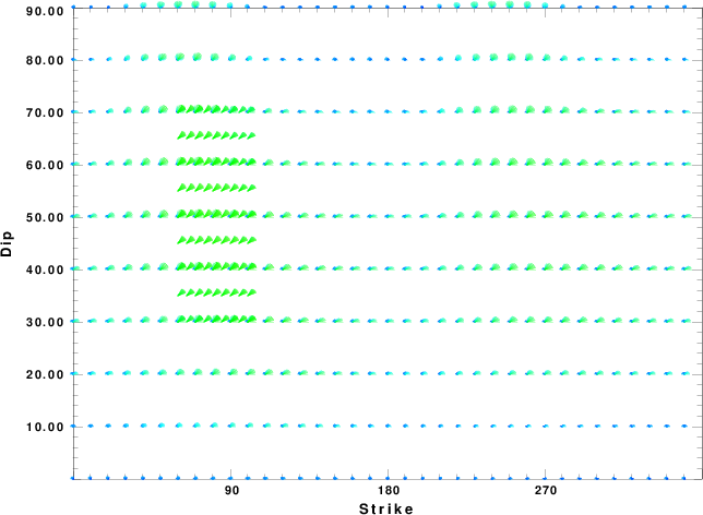
| Focal mechanism sensitivity at the preferred depth. The red color indicates a very good fit to the waveforms. Each solution is plotted as a vector at a given value of strike and dip with the angle of the vector representing the rake angle, measured, with respect to the upward vertical (N) in the figure. |
A check on the assumed source location is possible by looking at the time shifts between the observed and predicted traces. The time shifts for waveform matching arise for several reasons:
Time_shift = A + B cos Azimuth + C Sin Azimuth
The time shifts for this inversion lead to the next figure:
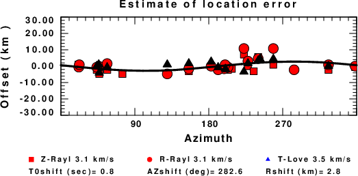
The derived shift in origin time and epicentral coordinates are given at the bottom of the figure.
The WUS.model used for the waveform synthetic seismograms and for the surface wave eigenfunctions and dispersion is as follows (The format is in the model96 format of Computer Programs in Seismology).
MODEL.01
Model after     8 iterations
ISOTROPIC
KGS
FLAT EARTH
1-D
CONSTANT VELOCITY
LINE08
LINE09
LINE10
LINE11
      H(KM)   VP(KM/S)   VS(KM/S) RHO(GM/CC)         QP         QS       ETAP       ETAS      FREFP      FREFS
     1.9000     3.4065     2.0089     2.2150  0.302E-02  0.679E-02   0.00       0.00       1.00       1.00
     6.1000     5.5445     3.2953     2.6089  0.349E-02  0.784E-02   0.00       0.00       1.00       1.00
    13.0000     6.2708     3.7396     2.7812  0.212E-02  0.476E-02   0.00       0.00       1.00       1.00
    19.0000     6.4075     3.7680     2.8223  0.111E-02  0.249E-02   0.00       0.00       1.00       1.00
     0.0000     7.9000     4.6200     3.2760  0.164E-10  0.370E-10   0.00       0.00       1.00       1.00