Location
Location ANSS
The ANSS event ID is ak016anz0nt3 and the event page is at
https://earthquake.usgs.gov/earthquakes/eventpage/ak016anz0nt3/executive.
2016/08/19 17:36:28 61.600 -146.336 23.9 4.3 Alaska
Focal Mechanism
 USGS/SLU Moment Tensor Solution
 ENS  2016/08/19 17:36:28:0  61.60 -146.34  23.9 4.3 Alaska

 Stations used:
   AK.BERG AK.BMR AK.CUT AK.DHY AK.DIV AK.EYAK AK.FID AK.GHO
   AK.GLI AK.HIN AK.HMT AK.KLU AK.KNK AK.MCAR AK.PAX AK.PWL
   AK.RAG AK.RC01 AK.SAW AK.SCM AK.TGL AT.PMR TA.M24K TA.M26K
   TA.N25K

 Filtering commands used:
   cut o DIST/3.3 -30 o DIST/3.3 +70
   rtr
   taper w 0.1
   hp c 0.03 n 3
   lp c 0.08 n 3

 Best Fitting Double Couple
  Mo = 3.55e+22 dyne-cm
  Mw = 4.30
  Z  = 41 km
  Plane   Strike  Dip  Rake
   NP1       50    70   -70
   NP2      183    28   -133
  Principal Axes:
   Axis    Value   Plunge  Azimuth
    T   3.55e+22     22     125
    N   0.00e+00     19     223
    P  -3.55e+22     60     349

 Moment Tensor: (dyne-cm)
    Component   Value
       Mxx     1.35e+21
       Mxy    -1.25e+22
       Mxz    -2.22e+22
       Myy     2.01e+22
       Myz     1.32e+22
       Mzz    -2.14e+22


                     ####----------
                 #####-----------------
              ######----------------------
             #####-------------------------
           ######---------------------------#
          #####----------   ---------------###
         ######---------- P --------------#####
        ######-----------   -------------#######
        #####--------------------------#########
       ######-------------------------###########
       ######-----------------------#############
       ######----------------------##############
       ######--------------------################
        #####-----------------##################
        ######--------------####################
         #####-----------###############   ####
          #####-------################## T ###
           #####--######################   ##
             ----##########################
              -----#######################
                 ----##################
                     ---###########


 Global CMT Convention Moment Tensor:
      R          T          P
 -2.14e+22  -2.22e+22  -1.32e+22
 -2.22e+22   1.35e+21   1.25e+22
 -1.32e+22   1.25e+22   2.01e+22


Details of the solution is found at

http://www.eas.slu.edu/eqc/eqc_mt/MECH.NA/20160819173628/index.html
|
Preferred Solution
The preferred solution from an analysis of the surface-wave spectral amplitude radiation pattern, waveform inversion or first motion observations is
      STK = 50
      DIP = 70
     RAKE = -70
       MW = 4.30
       HS = 41.0
The NDK file is 20160819173628.ndk
The waveform inversion is preferred.
Moment Tensor Comparison
The following compares this source inversion to those provided by others. The purpose is to look for major differences and also to note slight differences that might be inherent to the processing procedure. For completeness the USGS/SLU solution is repeated from above.
| SLU |
USGSMT |
 USGS/SLU Moment Tensor Solution
 ENS  2016/08/19 17:36:28:0  61.60 -146.34  23.9 4.3 Alaska

 Stations used:
   AK.BERG AK.BMR AK.CUT AK.DHY AK.DIV AK.EYAK AK.FID AK.GHO
   AK.GLI AK.HIN AK.HMT AK.KLU AK.KNK AK.MCAR AK.PAX AK.PWL
   AK.RAG AK.RC01 AK.SAW AK.SCM AK.TGL AT.PMR TA.M24K TA.M26K
   TA.N25K

 Filtering commands used:
   cut o DIST/3.3 -30 o DIST/3.3 +70
   rtr
   taper w 0.1
   hp c 0.03 n 3
   lp c 0.08 n 3

 Best Fitting Double Couple
  Mo = 3.55e+22 dyne-cm
  Mw = 4.30
  Z  = 41 km
  Plane   Strike  Dip  Rake
   NP1       50    70   -70
   NP2      183    28   -133
  Principal Axes:
   Axis    Value   Plunge  Azimuth
    T   3.55e+22     22     125
    N   0.00e+00     19     223
    P  -3.55e+22     60     349

 Moment Tensor: (dyne-cm)
    Component   Value
       Mxx     1.35e+21
       Mxy    -1.25e+22
       Mxz    -2.22e+22
       Myy     2.01e+22
       Myz     1.32e+22
       Mzz    -2.14e+22


                     ####----------
                 #####-----------------
              ######----------------------
             #####-------------------------
           ######---------------------------#
          #####----------   ---------------###
         ######---------- P --------------#####
        ######-----------   -------------#######
        #####--------------------------#########
       ######-------------------------###########
       ######-----------------------#############
       ######----------------------##############
       ######--------------------################
        #####-----------------##################
        ######--------------####################
         #####-----------###############   ####
          #####-------################## T ###
           #####--######################   ##
             ----##########################
              -----#######################
                 ----##################
                     ---###########


 Global CMT Convention Moment Tensor:
      R          T          P
 -2.14e+22  -2.22e+22  -1.32e+22
 -2.22e+22   1.35e+21   1.25e+22
 -1.32e+22   1.25e+22   2.01e+22


Details of the solution is found at

http://www.eas.slu.edu/eqc/eqc_mt/MECH.NA/20160819173628/index.html
|
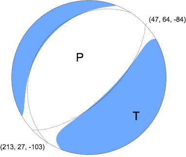
Regional Moment Tensor (Mwr)
Moment	4.051e+15 N-m
Magnitude	4.3 Mwr
Depth	43.0 km
Percent DC	82 %
Half Duration	–
Catalog	US
Data Source	US3
Contributor	US3
Nodal Planes
Plane	Strike	Dip	Rake
NP1	47	64	-84
NP2	213	27	-103
Principal Axes
Axis	Value	Plunge	Azimuth
T	4.232e+15 N-m	19	132
N	-0.391e+15 N-m	6	224
P	-3.841e+15 N-m	70	330
|
Magnitudes
Given the availability of digital waveforms for determination of the moment tensor, this section documents the added processing leading to mLg, if appropriate to the region, and ML by application of the respective IASPEI formulae. As a research study, the linear distance term of the IASPEI formula
for ML is adjusted to remove a linear distance trend in residuals to give a regionally defined ML. The defined ML uses horizontal component recordings, but the same procedure is applied to the vertical components since there may be some interest in vertical component ground motions. Residual plots versus distance may indicate interesting features of ground motion scaling in some distance ranges. A residual plot of the regionalized magnitude is given as a function of distance and azimuth, since data sets may transcend different wave propagation provinces.
ML Magnitude
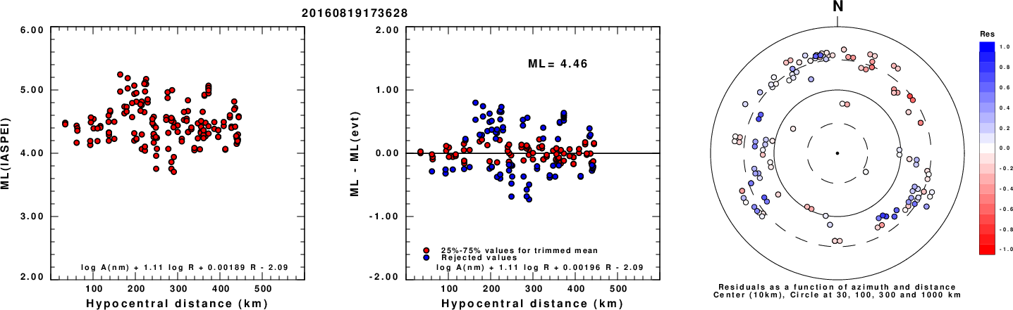
Left: ML computed using the IASPEI formula for Horizontal components. Center: ML residuals computed using a modified IASPEI formula that accounts for path specific attenuation; the values used for the trimmed mean are indicated. The ML relation used for each figure is given at the bottom of each plot.
Right: Residuals from new relation as a function of distance and azimuth.
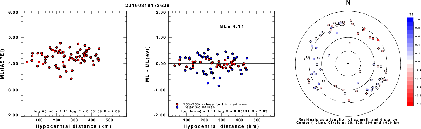
Left: ML computed using the IASPEI formula for Vertical components (research). Center: ML residuals computed using a modified IASPEI formula that accounts for path specific attenuation; the values used for the trimmed mean are indicated. The ML relation used for each figure is given at the bottom of each plot.
Right: Residuals from new relation as a function of distance and azimuth.
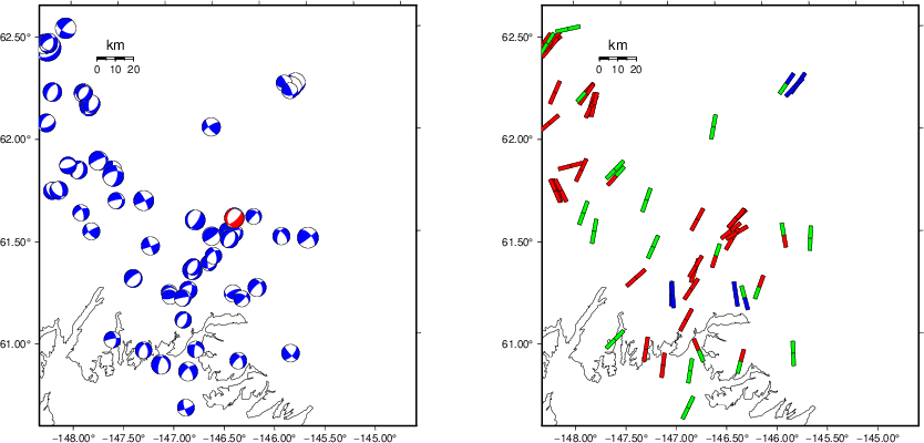
Context
The left panel of the next figure presents the focal mechanism for this earthquake (red) in the context of other nearby events (blue) in the SLU Moment Tensor Catalog. The right panel shows the inferred direction of maximum compressive stress and the type of faulting (green is strike-slip, red is normal, blue is thrust; oblique is shown by a combination of colors). Thus context plot is useful for assessing the appropriateness of the moment tensor of this event.
Waveform Inversion using wvfgrd96
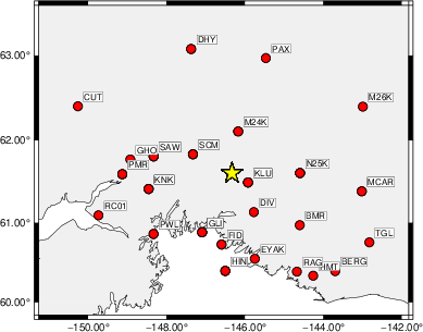
The focal mechanism was determined using broadband seismic waveforms. The location of the event (star) and the
stations used for (red) the waveform inversion are shown in the next figure.
|
|
Location of broadband stations used for waveform inversion
|
The program wvfgrd96 was used with good traces observed at short distance to determine the focal mechanism, depth and seismic moment. This technique requires a high quality signal and well determined velocity model for the Green's functions. To the extent that these are the quality data, this type of mechanism should be preferred over the radiation pattern technique which requires the separate step of defining the pressure and tension quadrants and the correct strike.
The observed and predicted traces are filtered using the following gsac commands:
cut o DIST/3.3 -30 o DIST/3.3 +70
rtr
taper w 0.1
hp c 0.03 n 3
lp c 0.08 n 3
The results of this grid search are as follow:
           DEPTH  STK   DIP  RAKE   MW    FIT
WVFGRD96    1.0   220    45    90   3.50 0.1923
WVFGRD96    2.0    35    45   -95   3.64 0.2681
WVFGRD96    3.0    30    45  -100   3.71 0.2834
WVFGRD96    4.0   225    50   -80   3.73 0.2707
WVFGRD96    5.0   250    55   -35   3.69 0.2641
WVFGRD96    6.0   210    80    55   3.70 0.2895
WVFGRD96    7.0   215    75    55   3.72 0.3115
WVFGRD96    8.0   225    75    65   3.81 0.3319
WVFGRD96    9.0   220    75    60   3.81 0.3495
WVFGRD96   10.0   220    75    60   3.82 0.3649
WVFGRD96   11.0   220    75    60   3.84 0.3769
WVFGRD96   12.0   215    75    60   3.84 0.3874
WVFGRD96   13.0   215    75    60   3.85 0.3963
WVFGRD96   14.0   300    40    20   3.87 0.4048
WVFGRD96   15.0   300    40    20   3.88 0.4134
WVFGRD96   16.0   300    40    20   3.89 0.4215
WVFGRD96   17.0   300    40    20   3.91 0.4289
WVFGRD96   18.0   280    35   -25   3.92 0.4409
WVFGRD96   19.0   275    35   -30   3.93 0.4501
WVFGRD96   20.0   270    35   -30   3.94 0.4591
WVFGRD96   21.0   280    35   -25   3.96 0.4671
WVFGRD96   22.0   270    30   -30   3.97 0.4771
WVFGRD96   23.0   270    30   -30   3.98 0.4862
WVFGRD96   24.0   265    30   -40   4.00 0.4956
WVFGRD96   25.0   265    30   -40   4.01 0.5044
WVFGRD96   26.0    65    75   -60   4.05 0.5220
WVFGRD96   27.0    65    75   -55   4.07 0.5361
WVFGRD96   28.0    60    70   -60   4.08 0.5494
WVFGRD96   29.0    60    70   -60   4.09 0.5630
WVFGRD96   30.0    60    70   -60   4.10 0.5751
WVFGRD96   31.0    60    70   -60   4.11 0.5868
WVFGRD96   32.0    60    70   -60   4.12 0.5968
WVFGRD96   33.0    60    70   -60   4.13 0.6056
WVFGRD96   34.0    60    70   -60   4.14 0.6113
WVFGRD96   35.0    60    70   -55   4.15 0.6162
WVFGRD96   36.0    60    70   -55   4.16 0.6187
WVFGRD96   37.0    55    70   -65   4.16 0.6198
WVFGRD96   38.0    55    70   -65   4.17 0.6227
WVFGRD96   39.0    55    70   -65   4.17 0.6241
WVFGRD96   40.0    50    70   -70   4.29 0.6453
WVFGRD96   41.0    50    70   -70   4.30 0.6454
WVFGRD96   42.0    50    70   -70   4.31 0.6432
WVFGRD96   43.0    50    70   -70   4.32 0.6417
WVFGRD96   44.0    50    70   -70   4.32 0.6385
WVFGRD96   45.0    45    65   -75   4.33 0.6350
WVFGRD96   46.0    45    65   -75   4.34 0.6337
WVFGRD96   47.0    45    65   -75   4.34 0.6313
WVFGRD96   48.0    55    70   -60   4.35 0.6287
WVFGRD96   49.0    45    65   -75   4.35 0.6269
WVFGRD96   50.0    55    70   -60   4.36 0.6244
WVFGRD96   51.0    50    70   -65   4.37 0.6213
WVFGRD96   52.0    50    70   -65   4.37 0.6207
WVFGRD96   53.0    50    70   -65   4.38 0.6185
WVFGRD96   54.0    45    65   -75   4.38 0.6179
WVFGRD96   55.0    45    65   -75   4.38 0.6162
WVFGRD96   56.0    45    65   -75   4.39 0.6142
WVFGRD96   57.0    45    65   -75   4.39 0.6114
WVFGRD96   58.0    45    65   -75   4.39 0.6085
WVFGRD96   59.0    45    65   -75   4.39 0.6052
WVFGRD96   60.0    45    65   -75   4.40 0.6010
WVFGRD96   61.0    45    65   -75   4.40 0.5964
WVFGRD96   62.0    45    65   -75   4.40 0.5918
WVFGRD96   63.0    45    65   -75   4.40 0.5864
WVFGRD96   64.0    45    65   -75   4.40 0.5808
WVFGRD96   65.0    45    65   -75   4.40 0.5739
WVFGRD96   66.0    45    65   -75   4.40 0.5678
WVFGRD96   67.0    50    70   -70   4.41 0.5606
WVFGRD96   68.0    50    70   -70   4.41 0.5540
WVFGRD96   69.0    45    70   -80   4.41 0.5477
WVFGRD96   70.0    45    75   -80   4.42 0.5425
WVFGRD96   71.0    45    75   -80   4.42 0.5397
WVFGRD96   72.0    45    75   -80   4.42 0.5354
WVFGRD96   73.0    45    75   -80   4.42 0.5322
WVFGRD96   74.0    45    75   -80   4.42 0.5285
WVFGRD96   75.0    45    75   -80   4.42 0.5241
WVFGRD96   76.0   260    20   -45   4.42 0.5212
WVFGRD96   77.0   260    20   -45   4.43 0.5182
WVFGRD96   78.0   260    20   -45   4.43 0.5156
WVFGRD96   79.0   260    20   -45   4.43 0.5106
WVFGRD96   80.0   265    25   -40   4.43 0.5047
WVFGRD96   81.0   265    25   -40   4.43 0.5002
WVFGRD96   82.0   265    25   -40   4.43 0.4931
WVFGRD96   83.0   265    25   -40   4.43 0.4856
WVFGRD96   84.0   265    25   -40   4.43 0.4776
WVFGRD96   85.0   260    25   -45   4.43 0.4689
WVFGRD96   86.0   260    25   -45   4.43 0.4602
WVFGRD96   87.0   265    25   -35   4.43 0.4528
WVFGRD96   88.0   270    25   -30   4.43 0.4502
WVFGRD96   89.0   270    25   -30   4.43 0.4477
WVFGRD96   90.0   270    25   -30   4.43 0.4464
WVFGRD96   91.0   270    25   -30   4.43 0.4441
WVFGRD96   92.0   270    25   -30   4.44 0.4404
WVFGRD96   93.0   270    25   -30   4.44 0.4366
WVFGRD96   94.0   275    25   -25   4.44 0.4321
WVFGRD96   95.0   275    25   -25   4.44 0.4256
WVFGRD96   96.0   280    25   -25   4.44 0.4194
WVFGRD96   97.0   285    25   -20   4.44 0.4127
WVFGRD96   98.0   285    25   -20   4.44 0.4046
WVFGRD96   99.0   290    25   -15   4.44 0.3963
The best solution is
WVFGRD96 41.0 50 70 -70 4.30 0.6454
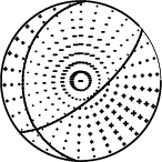
The mechanism corresponding to the best fit is
|
|
Figure 1. Waveform inversion focal mechanism
|
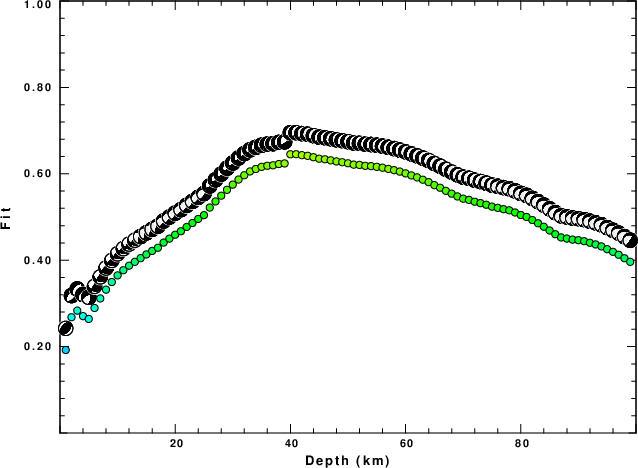
The best fit as a function of depth is given in the following figure:
|
|
Figure 2. Depth sensitivity for waveform mechanism
|
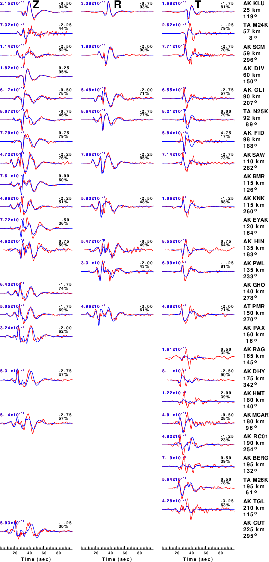
The comparison of the observed and predicted waveforms is given in the next figure. The red traces are the observed and the blue are the predicted.
Each observed-predicted component is plotted to the same scale and peak amplitudes are indicated by the numbers to the left of each trace. A pair of numbers is given in black at the right of each predicted traces. The upper number it the time shift required for maximum correlation between the observed and predicted traces. This time shift is required because the synthetics are not computed at exactly the same distance as the observed, the velocity model used in the predictions may not be perfect and the epicentral parameters may be be off.
A positive time shift indicates that the prediction is too fast and should be delayed to match the observed trace (shift to the right in this figure). A negative value indicates that the prediction is too slow. The lower number gives the percentage of variance reduction to characterize the individual goodness of fit (100% indicates a perfect fit).
The bandpass filter used in the processing and for the display was
cut o DIST/3.3 -30 o DIST/3.3 +70
rtr
taper w 0.1
hp c 0.03 n 3
lp c 0.08 n 3
|
|
Figure 3. Waveform comparison for selected depth. Red: observed; Blue - predicted. The time shift with respect to the model prediction is indicated. The percent of fit is also indicated. The time scale is relative to the first trace sample.
|
|
|
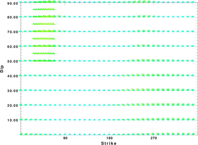
Focal mechanism sensitivity at the preferred depth. The red color indicates a very good fit to the waveforms.
Each solution is plotted as a vector at a given value of strike and dip with the angle of the vector representing the rake angle, measured, with respect to the upward vertical (N) in the figure.
|
A check on the assumed source location is possible by looking at the time shifts between the observed and predicted traces. The time shifts for waveform matching arise for several reasons:
- The origin time and epicentral distance are incorrect
- The velocity model used for the inversion is incorrect
- The velocity model used to define the P-arrival time is not the
same as the velocity model used for the waveform inversion
(assuming that the initial trace alignment is based on the
P arrival time)
Assuming only a mislocation, the time shifts are fit to a functional form:
Time_shift = A + B cos Azimuth + C Sin Azimuth
The time shifts for this inversion lead to the next figure:
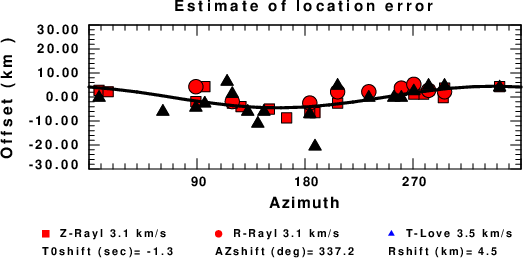
The derived shift in origin time and epicentral coordinates are given at the bottom of the figure.
Velocity Model
The WUS.model used for the waveform synthetic seismograms and for the surface wave eigenfunctions and dispersion is as follows
(The format is in the model96 format of Computer Programs in Seismology).
MODEL.01
Model after     8 iterations
ISOTROPIC
KGS
FLAT EARTH
1-D
CONSTANT VELOCITY
LINE08
LINE09
LINE10
LINE11
      H(KM)   VP(KM/S)   VS(KM/S) RHO(GM/CC)         QP         QS       ETAP       ETAS      FREFP      FREFS
     1.9000     3.4065     2.0089     2.2150  0.302E-02  0.679E-02   0.00       0.00       1.00       1.00
     6.1000     5.5445     3.2953     2.6089  0.349E-02  0.784E-02   0.00       0.00       1.00       1.00
    13.0000     6.2708     3.7396     2.7812  0.212E-02  0.476E-02   0.00       0.00       1.00       1.00
    19.0000     6.4075     3.7680     2.8223  0.111E-02  0.249E-02   0.00       0.00       1.00       1.00
     0.0000     7.9000     4.6200     3.2760  0.164E-10  0.370E-10   0.00       0.00       1.00       1.00
Last Changed Fri Apr 26 08:05:50 PM CDT 2024