Location
Location ANSS
The ANSS event ID is ak0169vkoz7q and the event page is at
https://earthquake.usgs.gov/earthquakes/eventpage/ak0169vkoz7q/executive.
2016/08/02 00:25:01 62.049 -149.391 38.2 4.1 Alaska
Focal Mechanism
USGS/SLU Moment Tensor Solution
ENS 2016/08/02 00:25:01:0 62.05 -149.39 38.2 4.1 Alaska
Stations used:
AK.CUT AK.DHY AK.GHO AK.GLI AK.HDA AK.HIN AK.KNK AK.PWL
AK.RC01 AK.SAW AK.SCM AK.WRH AT.PMR TA.J20K TA.M22K TA.N25K
TA.O22K
Filtering commands used:
cut o DIST/3.3 -40 o DIST/3.3 +30
rtr
taper w 0.1
hp c 0.03 n 3
lp c 0.10 n 3
Best Fitting Double Couple
Mo = 1.72e+22 dyne-cm
Mw = 4.09
Z = 52 km
Plane Strike Dip Rake
NP1 336 52 -117
NP2 195 45 -60
Principal Axes:
Axis Value Plunge Azimuth
T 1.72e+22 4 84
N 0.00e+00 21 353
P -1.72e+22 69 184
Moment Tensor: (dyne-cm)
Component Value
Mxx -2.04e+21
Mxy 1.54e+21
Mxz 5.87e+21
Myy 1.69e+22
Myz 1.57e+21
Mzz -1.49e+22
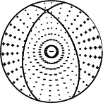
----------####
#######---############
###########--###############
##########-------#############
##########----------##############
##########-------------#############
##########---------------#############
##########-----------------#############
##########------------------##########
##########--------------------######### T
##########---------------------########
#########----------------------###########
#########-----------------------##########
########---------- ----------#########
########---------- P ----------#########
########--------- ----------########
#######----------------------#######
######----------------------######
#####---------------------####
#####-------------------####
###-----------------##
#-------------
Global CMT Convention Moment Tensor:
R T P
-1.49e+22 5.87e+21 -1.57e+21
5.87e+21 -2.04e+21 -1.54e+21
-1.57e+21 -1.54e+21 1.69e+22
Details of the solution is found at
http://www.eas.slu.edu/eqc/eqc_mt/MECH.NA/20160802002501/index.html
|
Preferred Solution
The preferred solution from an analysis of the surface-wave spectral amplitude radiation pattern, waveform inversion or first motion observations is
      STK = 195
      DIP = 45
     RAKE = -60
       MW = 4.09
       HS = 52.0
The NDK file is 20160802002501.ndk
The waveform inversion is preferred.
Magnitudes
Given the availability of digital waveforms for determination of the moment tensor, this section documents the added processing leading to mLg, if appropriate to the region, and ML by application of the respective IASPEI formulae. As a research study, the linear distance term of the IASPEI formula
for ML is adjusted to remove a linear distance trend in residuals to give a regionally defined ML. The defined ML uses horizontal component recordings, but the same procedure is applied to the vertical components since there may be some interest in vertical component ground motions. Residual plots versus distance may indicate interesting features of ground motion scaling in some distance ranges. A residual plot of the regionalized magnitude is given as a function of distance and azimuth, since data sets may transcend different wave propagation provinces.
ML Magnitude
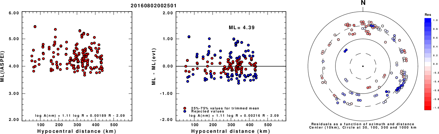
Left: ML computed using the IASPEI formula for Horizontal components. Center: ML residuals computed using a modified IASPEI formula that accounts for path specific attenuation; the values used for the trimmed mean are indicated. The ML relation used for each figure is given at the bottom of each plot.
Right: Residuals from new relation as a function of distance and azimuth.
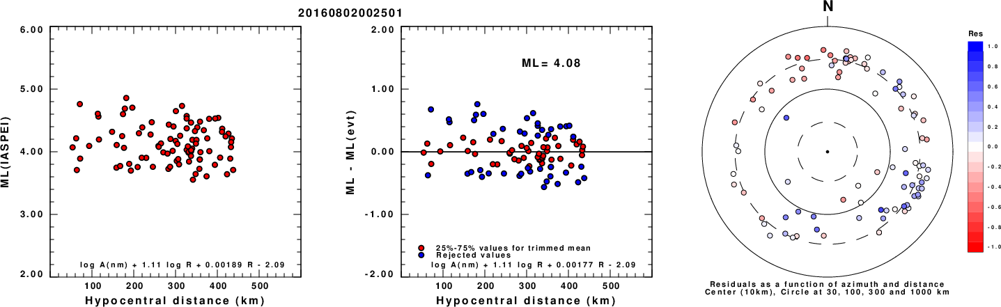
Left: ML computed using the IASPEI formula for Vertical components (research). Center: ML residuals computed using a modified IASPEI formula that accounts for path specific attenuation; the values used for the trimmed mean are indicated. The ML relation used for each figure is given at the bottom of each plot.
Right: Residuals from new relation as a function of distance and azimuth.
Context
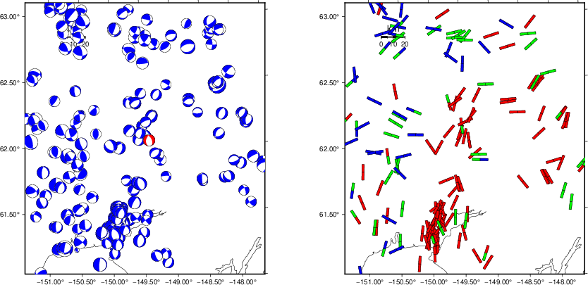
The left panel of the next figure presents the focal mechanism for this earthquake (red) in the context of other nearby events (blue) in the SLU Moment Tensor Catalog. The right panel shows the inferred direction of maximum compressive stress and the type of faulting (green is strike-slip, red is normal, blue is thrust; oblique is shown by a combination of colors). Thus context plot is useful for assessing the appropriateness of the moment tensor of this event.
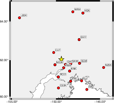
Waveform Inversion using wvfgrd96
The focal mechanism was determined using broadband seismic waveforms. The location of the event (star) and the
stations used for (red) the waveform inversion are shown in the next figure.
|
|
Location of broadband stations used for waveform inversion
|
The program wvfgrd96 was used with good traces observed at short distance to determine the focal mechanism, depth and seismic moment. This technique requires a high quality signal and well determined velocity model for the Green's functions. To the extent that these are the quality data, this type of mechanism should be preferred over the radiation pattern technique which requires the separate step of defining the pressure and tension quadrants and the correct strike.
The observed and predicted traces are filtered using the following gsac commands:
cut o DIST/3.3 -40 o DIST/3.3 +30
rtr
taper w 0.1
hp c 0.03 n 3
lp c 0.10 n 3
The results of this grid search are as follow:
           DEPTH  STK   DIP  RAKE   MW    FIT
WVFGRD96    1.0   185    40    90   3.18 0.2201
WVFGRD96    2.0    -5    50    85   3.33 0.2746
WVFGRD96    3.0   320    20    50   3.38 0.2450
WVFGRD96    4.0   320    20    45   3.38 0.2873
WVFGRD96    5.0   320    25    45   3.38 0.3098
WVFGRD96    6.0   320    25    45   3.39 0.3265
WVFGRD96    7.0   325    25    55   3.41 0.3390
WVFGRD96    8.0   330    20    60   3.49 0.3452
WVFGRD96    9.0   335    20    65   3.50 0.3527
WVFGRD96   10.0   335    20    70   3.53 0.3618
WVFGRD96   11.0   335    20    70   3.54 0.3677
WVFGRD96   12.0   330    25    65   3.55 0.3697
WVFGRD96   13.0   330    25    65   3.57 0.3703
WVFGRD96   14.0   330    25    65   3.58 0.3677
WVFGRD96   15.0   345    25    80   3.59 0.3636
WVFGRD96   16.0   340    25    75   3.60 0.3580
WVFGRD96   17.0   340    25    75   3.61 0.3509
WVFGRD96   18.0   330    25    65   3.62 0.3423
WVFGRD96   19.0   330    25    65   3.63 0.3336
WVFGRD96   20.0    25    45   -40   3.64 0.3280
WVFGRD96   21.0    25    45   -45   3.66 0.3303
WVFGRD96   22.0    25    40   -45   3.67 0.3310
WVFGRD96   23.0    25    40   -45   3.68 0.3319
WVFGRD96   24.0    25    40   -45   3.69 0.3312
WVFGRD96   25.0    25    40   -45   3.70 0.3277
WVFGRD96   26.0    20    40   -55   3.70 0.3227
WVFGRD96   27.0   240    40   -25   3.74 0.3204
WVFGRD96   28.0   245    35   -20   3.76 0.3358
WVFGRD96   29.0   240    35   -30   3.77 0.3523
WVFGRD96   30.0   240    35   -30   3.78 0.3670
WVFGRD96   31.0   240    35   -30   3.79 0.3832
WVFGRD96   32.0   175    40   -85   3.80 0.4087
WVFGRD96   33.0   175    40   -85   3.81 0.4448
WVFGRD96   34.0   175    40   -85   3.83 0.4758
WVFGRD96   35.0   180    40   -80   3.84 0.5060
WVFGRD96   36.0   180    40   -80   3.85 0.5370
WVFGRD96   37.0   180    40   -80   3.86 0.5623
WVFGRD96   38.0   180    40   -75   3.89 0.5842
WVFGRD96   39.0   180    40   -75   3.90 0.6013
WVFGRD96   40.0   185    40   -75   3.98 0.6134
WVFGRD96   41.0   185    40   -75   3.99 0.6141
WVFGRD96   42.0   185    40   -70   4.01 0.6193
WVFGRD96   43.0   185    40   -70   4.02 0.6232
WVFGRD96   44.0   185    40   -70   4.03 0.6269
WVFGRD96   45.0   185    40   -70   4.04 0.6320
WVFGRD96   46.0   185    40   -70   4.05 0.6347
WVFGRD96   47.0   185    40   -70   4.05 0.6380
WVFGRD96   48.0   190    40   -65   4.06 0.6387
WVFGRD96   49.0   190    40   -65   4.07 0.6405
WVFGRD96   50.0   185    40   -65   4.08 0.6400
WVFGRD96   51.0   195    45   -60   4.08 0.6401
WVFGRD96   52.0   195    45   -60   4.09 0.6408
WVFGRD96   53.0   195    45   -60   4.09 0.6387
WVFGRD96   54.0   195    45   -60   4.09 0.6387
WVFGRD96   55.0   195    45   -55   4.10 0.6337
WVFGRD96   56.0   195    45   -55   4.11 0.6332
WVFGRD96   57.0   195    45   -55   4.11 0.6293
WVFGRD96   58.0   195    45   -55   4.11 0.6252
WVFGRD96   59.0   195    45   -55   4.11 0.6220
WVFGRD96   60.0   195    45   -55   4.11 0.6150
WVFGRD96   61.0   200    50   -50   4.12 0.6133
WVFGRD96   62.0   200    50   -50   4.12 0.6081
WVFGRD96   63.0   200    50   -50   4.12 0.6049
WVFGRD96   64.0   200    50   -50   4.12 0.6015
WVFGRD96   65.0   200    50   -50   4.12 0.5958
WVFGRD96   66.0   200    50   -50   4.12 0.5912
WVFGRD96   67.0   205    50   -45   4.13 0.5877
WVFGRD96   68.0   205    50   -45   4.13 0.5820
WVFGRD96   69.0   205    50   -45   4.13 0.5780
WVFGRD96   70.0   205    50   -45   4.13 0.5723
WVFGRD96   71.0   205    50   -45   4.13 0.5683
WVFGRD96   72.0   205    55   -45   4.14 0.5625
WVFGRD96   73.0   205    55   -45   4.14 0.5588
WVFGRD96   74.0   210    55   -40   4.15 0.5555
WVFGRD96   75.0   210    55   -40   4.15 0.5511
WVFGRD96   76.0   210    55   -40   4.15 0.5468
WVFGRD96   77.0   210    55   -40   4.15 0.5436
WVFGRD96   78.0   210    55   -40   4.15 0.5395
WVFGRD96   79.0   210    55   -40   4.15 0.5346
The best solution is
WVFGRD96 52.0 195 45 -60 4.09 0.6408
The mechanism corresponding to the best fit is
|
|
Figure 1. Waveform inversion focal mechanism
|
The best fit as a function of depth is given in the following figure:
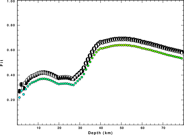
|
|
Figure 2. Depth sensitivity for waveform mechanism
|
The comparison of the observed and predicted waveforms is given in the next figure. The red traces are the observed and the blue are the predicted.
Each observed-predicted component is plotted to the same scale and peak amplitudes are indicated by the numbers to the left of each trace. A pair of numbers is given in black at the right of each predicted traces. The upper number it the time shift required for maximum correlation between the observed and predicted traces. This time shift is required because the synthetics are not computed at exactly the same distance as the observed, the velocity model used in the predictions may not be perfect and the epicentral parameters may be be off.
A positive time shift indicates that the prediction is too fast and should be delayed to match the observed trace (shift to the right in this figure). A negative value indicates that the prediction is too slow. The lower number gives the percentage of variance reduction to characterize the individual goodness of fit (100% indicates a perfect fit).
The bandpass filter used in the processing and for the display was
cut o DIST/3.3 -40 o DIST/3.3 +30
rtr
taper w 0.1
hp c 0.03 n 3
lp c 0.10 n 3
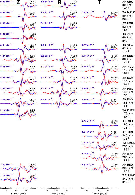
|
|
Figure 3. Waveform comparison for selected depth. Red: observed; Blue - predicted. The time shift with respect to the model prediction is indicated. The percent of fit is also indicated. The time scale is relative to the first trace sample.
|
|
|
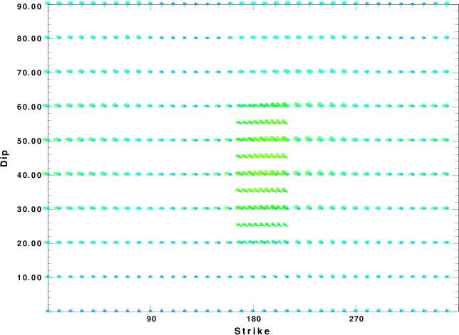
Focal mechanism sensitivity at the preferred depth. The red color indicates a very good fit to the waveforms.
Each solution is plotted as a vector at a given value of strike and dip with the angle of the vector representing the rake angle, measured, with respect to the upward vertical (N) in the figure.
|
A check on the assumed source location is possible by looking at the time shifts between the observed and predicted traces. The time shifts for waveform matching arise for several reasons:
- The origin time and epicentral distance are incorrect
- The velocity model used for the inversion is incorrect
- The velocity model used to define the P-arrival time is not the
same as the velocity model used for the waveform inversion
(assuming that the initial trace alignment is based on the
P arrival time)
Assuming only a mislocation, the time shifts are fit to a functional form:
Time_shift = A + B cos Azimuth + C Sin Azimuth
The time shifts for this inversion lead to the next figure:
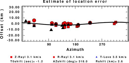
The derived shift in origin time and epicentral coordinates are given at the bottom of the figure.
Velocity Model
The WUS.model used for the waveform synthetic seismograms and for the surface wave eigenfunctions and dispersion is as follows
(The format is in the model96 format of Computer Programs in Seismology).
MODEL.01
Model after     8 iterations
ISOTROPIC
KGS
FLAT EARTH
1-D
CONSTANT VELOCITY
LINE08
LINE09
LINE10
LINE11
      H(KM)   VP(KM/S)   VS(KM/S) RHO(GM/CC)         QP         QS       ETAP       ETAS      FREFP      FREFS
     1.9000     3.4065     2.0089     2.2150  0.302E-02  0.679E-02   0.00       0.00       1.00       1.00
     6.1000     5.5445     3.2953     2.6089  0.349E-02  0.784E-02   0.00       0.00       1.00       1.00
    13.0000     6.2708     3.7396     2.7812  0.212E-02  0.476E-02   0.00       0.00       1.00       1.00
    19.0000     6.4075     3.7680     2.8223  0.111E-02  0.249E-02   0.00       0.00       1.00       1.00
     0.0000     7.9000     4.6200     3.2760  0.164E-10  0.370E-10   0.00       0.00       1.00       1.00
Last Changed Fri Apr 26 07:19:38 PM CDT 2024