Location
Location ANSS
The ANSS event ID is ak016690dapx and the event page is at
https://earthquake.usgs.gov/earthquakes/eventpage/ak016690dapx/executive.
2016/05/15 05:51:00 63.077 -150.946 131.5 5.3 Alaska
Focal Mechanism
 USGS/SLU Moment Tensor Solution
 ENS  2016/05/15 05:51:00:0  63.08 -150.95 131.5 5.3 Alaska

 Stations used:
   AK.BPAW AK.BWN AK.CAST AK.CCB AK.CUT AK.DHY AK.DIV AK.FID
   AK.FIRE AK.GHO AK.GLI AK.HDA AK.KLU AK.KNK AK.KTH AK.MCK
   AK.MDM AK.NEA2 AK.PAX AK.PPLA AK.RC01 AK.RND AK.SAW AK.SCM
   AK.TRF AK.WRH AT.PMR AT.SVW2 AT.TTA IM.IL31 IU.COLA TA.H21K
   TA.H23K TA.H24K TA.I21K TA.I23K TA.J20K TA.K20K TA.L19K
   TA.M19K TA.M22K TA.N19K TA.O22K TA.POKR TA.TCOL

 Filtering commands used:
   cut o DIST/3.3 -50 o DIST/3.3 +60
   rtr
   taper w 0.1
   hp c 0.03 n 3
   lp c 0.10 n 3

 Best Fitting Double Couple
  Mo = 9.12e+23 dyne-cm
  Mw = 5.24
  Z  = 126 km
  Plane   Strike  Dip  Rake
   NP1       50    60    65
   NP2      273    38   126
  Principal Axes:
   Axis    Value   Plunge  Azimuth
    T   9.12e+23     65     274
    N   0.00e+00     21      63
    P  -9.12e+23     12     158

 Moment Tensor: (dyne-cm)
    Component   Value
       Mxx    -7.49e+23
       Mxy     2.95e+23
       Mxz     1.93e+23
       Myy     3.30e+22
       Myz    -4.13e+23
       Mzz     7.16e+23


                     --------------
                 ----------------------
              ----------------------------
             ------------------------------
           ----------#############----------#
          ------#######################-----##
         ----#############################-####
        ---###############################--####
        -################################-----##
       -############   #################-------##
       ############# T ################---------#
       #############   ###############-----------
       #############################-------------
        ##########################--------------
        ########################----------------
         #####################-----------------
          #################-------------------
           ###########-----------------------
             ------------------------------
              -------------------   ------
                 ---------------- P ---
                     ------------


 Global CMT Convention Moment Tensor:
      R          T          P
  7.16e+23   1.93e+23   4.13e+23
  1.93e+23  -7.49e+23  -2.95e+23
  4.13e+23  -2.95e+23   3.30e+22


Details of the solution is found at

http://www.eas.slu.edu/eqc/eqc_mt/MECH.NA/20160515055100/index.html
|
Preferred Solution
The preferred solution from an analysis of the surface-wave spectral amplitude radiation pattern, waveform inversion or first motion observations is
      STK = 50
      DIP = 60
     RAKE = 65
       MW = 5.24
       HS = 126.0
The NDK file is 20160515055100.ndk
The waveform inversion is preferred.
Moment Tensor Comparison
The following compares this source inversion to those provided by others. The purpose is to look for major differences and also to note slight differences that might be inherent to the processing procedure. For completeness the USGS/SLU solution is repeated from above.
| SLU |
USGSMT |
 USGS/SLU Moment Tensor Solution
 ENS  2016/05/15 05:51:00:0  63.08 -150.95 131.5 5.3 Alaska

 Stations used:
   AK.BPAW AK.BWN AK.CAST AK.CCB AK.CUT AK.DHY AK.DIV AK.FID
   AK.FIRE AK.GHO AK.GLI AK.HDA AK.KLU AK.KNK AK.KTH AK.MCK
   AK.MDM AK.NEA2 AK.PAX AK.PPLA AK.RC01 AK.RND AK.SAW AK.SCM
   AK.TRF AK.WRH AT.PMR AT.SVW2 AT.TTA IM.IL31 IU.COLA TA.H21K
   TA.H23K TA.H24K TA.I21K TA.I23K TA.J20K TA.K20K TA.L19K
   TA.M19K TA.M22K TA.N19K TA.O22K TA.POKR TA.TCOL

 Filtering commands used:
   cut o DIST/3.3 -50 o DIST/3.3 +60
   rtr
   taper w 0.1
   hp c 0.03 n 3
   lp c 0.10 n 3

 Best Fitting Double Couple
  Mo = 9.12e+23 dyne-cm
  Mw = 5.24
  Z  = 126 km
  Plane   Strike  Dip  Rake
   NP1       50    60    65
   NP2      273    38   126
  Principal Axes:
   Axis    Value   Plunge  Azimuth
    T   9.12e+23     65     274
    N   0.00e+00     21      63
    P  -9.12e+23     12     158

 Moment Tensor: (dyne-cm)
    Component   Value
       Mxx    -7.49e+23
       Mxy     2.95e+23
       Mxz     1.93e+23
       Myy     3.30e+22
       Myz    -4.13e+23
       Mzz     7.16e+23


                     --------------
                 ----------------------
              ----------------------------
             ------------------------------
           ----------#############----------#
          ------#######################-----##
         ----#############################-####
        ---###############################--####
        -################################-----##
       -############   #################-------##
       ############# T ################---------#
       #############   ###############-----------
       #############################-------------
        ##########################--------------
        ########################----------------
         #####################-----------------
          #################-------------------
           ###########-----------------------
             ------------------------------
              -------------------   ------
                 ---------------- P ---
                     ------------


 Global CMT Convention Moment Tensor:
      R          T          P
  7.16e+23   1.93e+23   4.13e+23
  1.93e+23  -7.49e+23  -2.95e+23
  4.13e+23  -2.95e+23   3.30e+22


Details of the solution is found at

http://www.eas.slu.edu/eqc/eqc_mt/MECH.NA/20160515055100/index.html
|
Body-wave Moment Tensor (Mwb)
Moment 1.053e+17 N-m
Magnitude 5.3 Mwb
Depth 130.0 km
Percent DC 87 %
Half Duration –
Catalog US
Data Source US3
Contributor US3
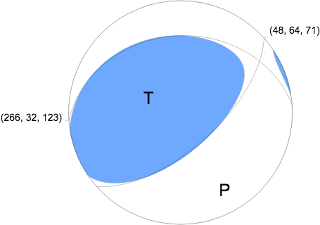
Nodal Planes
Plane Strike Dip Rake
NP1 266 32 123
NP2 48 64 71
Principal Axes
Axis Value Plunge Azimuth
T 1.087e+17 N-m 66 284
N -0.072e+17 N-m 17 57
P -1.015e+17 N-m 17 152
|
Magnitudes
Given the availability of digital waveforms for determination of the moment tensor, this section documents the added processing leading to mLg, if appropriate to the region, and ML by application of the respective IASPEI formulae. As a research study, the linear distance term of the IASPEI formula
for ML is adjusted to remove a linear distance trend in residuals to give a regionally defined ML. The defined ML uses horizontal component recordings, but the same procedure is applied to the vertical components since there may be some interest in vertical component ground motions. Residual plots versus distance may indicate interesting features of ground motion scaling in some distance ranges. A residual plot of the regionalized magnitude is given as a function of distance and azimuth, since data sets may transcend different wave propagation provinces.
ML Magnitude
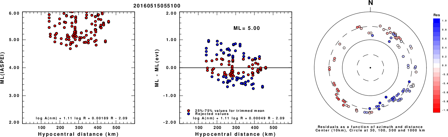
Left: ML computed using the IASPEI formula for Horizontal components. Center: ML residuals computed using a modified IASPEI formula that accounts for path specific attenuation; the values used for the trimmed mean are indicated. The ML relation used for each figure is given at the bottom of each plot.
Right: Residuals from new relation as a function of distance and azimuth.
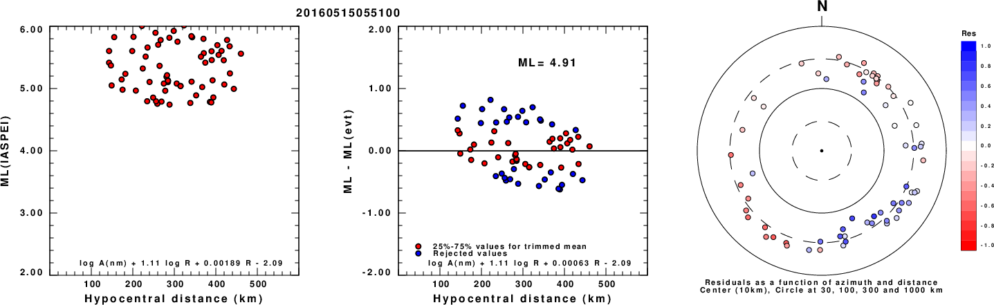
Left: ML computed using the IASPEI formula for Vertical components (research). Center: ML residuals computed using a modified IASPEI formula that accounts for path specific attenuation; the values used for the trimmed mean are indicated. The ML relation used for each figure is given at the bottom of each plot.
Right: Residuals from new relation as a function of distance and azimuth.
Context
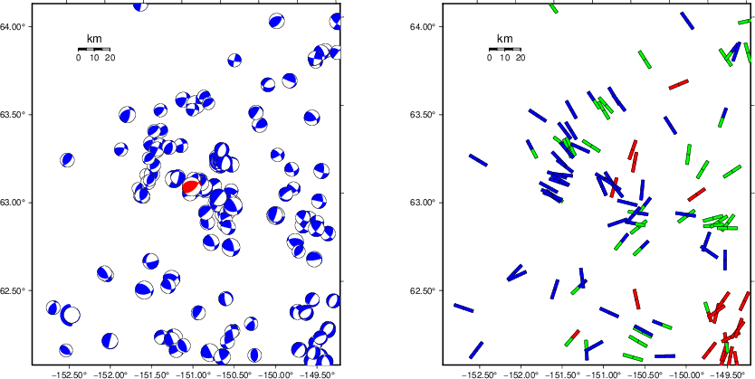
The left panel of the next figure presents the focal mechanism for this earthquake (red) in the context of other nearby events (blue) in the SLU Moment Tensor Catalog. The right panel shows the inferred direction of maximum compressive stress and the type of faulting (green is strike-slip, red is normal, blue is thrust; oblique is shown by a combination of colors). Thus context plot is useful for assessing the appropriateness of the moment tensor of this event.
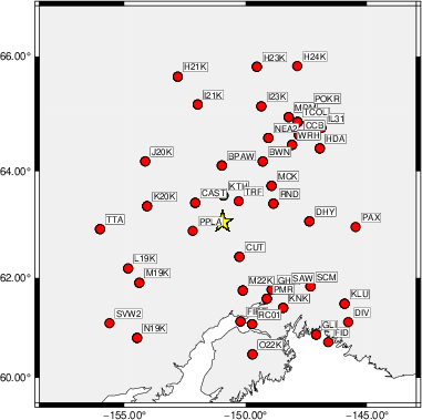
Waveform Inversion using wvfgrd96
The focal mechanism was determined using broadband seismic waveforms. The location of the event (star) and the
stations used for (red) the waveform inversion are shown in the next figure.
|
|
Location of broadband stations used for waveform inversion
|
The program wvfgrd96 was used with good traces observed at short distance to determine the focal mechanism, depth and seismic moment. This technique requires a high quality signal and well determined velocity model for the Green's functions. To the extent that these are the quality data, this type of mechanism should be preferred over the radiation pattern technique which requires the separate step of defining the pressure and tension quadrants and the correct strike.
The observed and predicted traces are filtered using the following gsac commands:
cut o DIST/3.3 -50 o DIST/3.3 +60
rtr
taper w 0.1
hp c 0.03 n 3
lp c 0.10 n 3
The results of this grid search are as follow:
           DEPTH  STK   DIP  RAKE   MW    FIT
WVFGRD96   70.0    55    50    65   5.11 0.3255
WVFGRD96   72.0    50    55    60   5.13 0.3645
WVFGRD96   74.0    50    55    60   5.14 0.4045
WVFGRD96   76.0    50    55    60   5.15 0.4459
WVFGRD96   78.0    50    55    60   5.17 0.4790
WVFGRD96   80.0    50    55    60   5.17 0.4992
WVFGRD96   82.0    50    55    60   5.18 0.5133
WVFGRD96   84.0    50    55    60   5.18 0.5258
WVFGRD96   86.0    50    55    60   5.18 0.5361
WVFGRD96   88.0    50    55    60   5.19 0.5452
WVFGRD96   90.0    50    60    65   5.19 0.5541
WVFGRD96   92.0    50    60    65   5.20 0.5611
WVFGRD96   94.0    50    60    65   5.20 0.5676
WVFGRD96   96.0    50    60    65   5.20 0.5734
WVFGRD96   98.0    50    60    65   5.21 0.5794
WVFGRD96  100.0    50    60    65   5.21 0.5841
WVFGRD96  102.0    50    60    65   5.21 0.5885
WVFGRD96  104.0    50    60    65   5.21 0.5920
WVFGRD96  106.0    50    60    65   5.22 0.5949
WVFGRD96  108.0    50    60    65   5.22 0.5991
WVFGRD96  110.0    50    60    65   5.22 0.6010
WVFGRD96  112.0    50    60    65   5.22 0.6038
WVFGRD96  114.0    50    60    65   5.23 0.6062
WVFGRD96  116.0    50    60    65   5.23 0.6078
WVFGRD96  118.0    50    60    65   5.23 0.6097
WVFGRD96  120.0    50    60    65   5.23 0.6111
WVFGRD96  122.0    50    60    65   5.23 0.6120
WVFGRD96  124.0    50    60    65   5.24 0.6122
WVFGRD96  126.0    50    60    65   5.24 0.6129
WVFGRD96  128.0    50    60    70   5.24 0.6121
WVFGRD96  130.0    50    60    70   5.24 0.6128
WVFGRD96  132.0    50    60    70   5.25 0.6113
WVFGRD96  134.0    50    60    70   5.25 0.6104
WVFGRD96  136.0    50    60    70   5.25 0.6090
WVFGRD96  138.0    50    60    70   5.25 0.6071
WVFGRD96  140.0    50    60    70   5.25 0.6059
WVFGRD96  142.0    50    60    70   5.25 0.6026
WVFGRD96  144.0    50    60    70   5.26 0.6011
WVFGRD96  146.0    50    55    65   5.26 0.5982
WVFGRD96  148.0    50    55    65   5.26 0.5956
The best solution is
WVFGRD96 126.0 50 60 65 5.24 0.6129
The mechanism corresponding to the best fit is
|
|
Figure 1. Waveform inversion focal mechanism
|
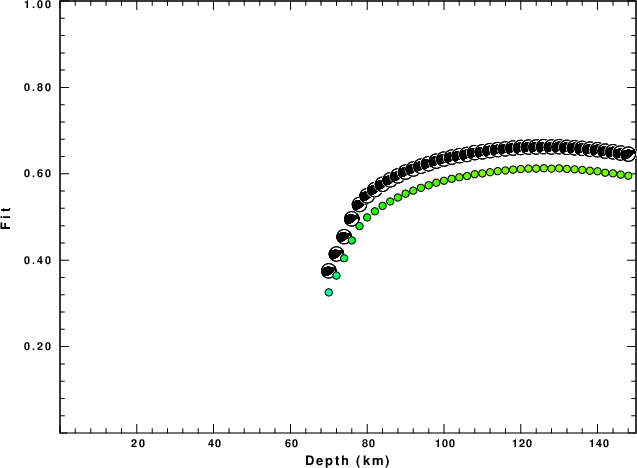
The best fit as a function of depth is given in the following figure:
|
|
Figure 2. Depth sensitivity for waveform mechanism
|
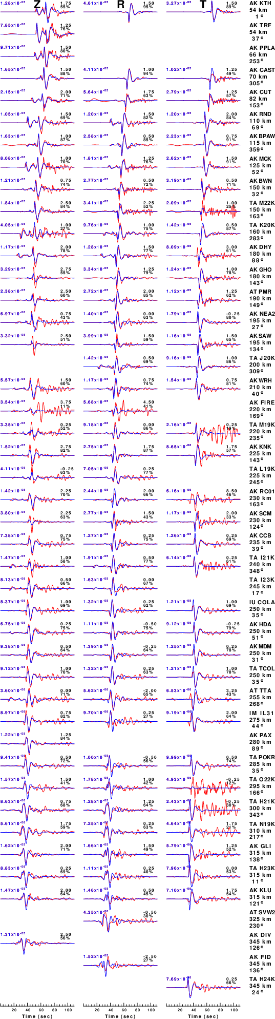
The comparison of the observed and predicted waveforms is given in the next figure. The red traces are the observed and the blue are the predicted.
Each observed-predicted component is plotted to the same scale and peak amplitudes are indicated by the numbers to the left of each trace. A pair of numbers is given in black at the right of each predicted traces. The upper number it the time shift required for maximum correlation between the observed and predicted traces. This time shift is required because the synthetics are not computed at exactly the same distance as the observed, the velocity model used in the predictions may not be perfect and the epicentral parameters may be be off.
A positive time shift indicates that the prediction is too fast and should be delayed to match the observed trace (shift to the right in this figure). A negative value indicates that the prediction is too slow. The lower number gives the percentage of variance reduction to characterize the individual goodness of fit (100% indicates a perfect fit).
The bandpass filter used in the processing and for the display was
cut o DIST/3.3 -50 o DIST/3.3 +60
rtr
taper w 0.1
hp c 0.03 n 3
lp c 0.10 n 3
|
|
Figure 3. Waveform comparison for selected depth. Red: observed; Blue - predicted. The time shift with respect to the model prediction is indicated. The percent of fit is also indicated. The time scale is relative to the first trace sample.
|
|
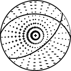
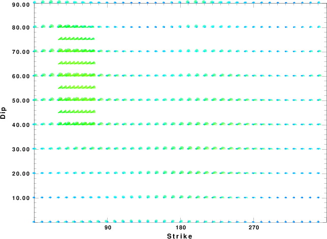
|
Focal mechanism sensitivity at the preferred depth. The red color indicates a very good fit to the waveforms.
Each solution is plotted as a vector at a given value of strike and dip with the angle of the vector representing the rake angle, measured, with respect to the upward vertical (N) in the figure.
|
A check on the assumed source location is possible by looking at the time shifts between the observed and predicted traces. The time shifts for waveform matching arise for several reasons:
- The origin time and epicentral distance are incorrect
- The velocity model used for the inversion is incorrect
- The velocity model used to define the P-arrival time is not the
same as the velocity model used for the waveform inversion
(assuming that the initial trace alignment is based on the
P arrival time)
Assuming only a mislocation, the time shifts are fit to a functional form:
Time_shift = A + B cos Azimuth + C Sin Azimuth
The time shifts for this inversion lead to the next figure:
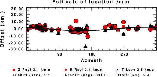
The derived shift in origin time and epicentral coordinates are given at the bottom of the figure.
Velocity Model
The WUS.model used for the waveform synthetic seismograms and for the surface wave eigenfunctions and dispersion is as follows
(The format is in the model96 format of Computer Programs in Seismology).
MODEL.01
Model after     8 iterations
ISOTROPIC
KGS
FLAT EARTH
1-D
CONSTANT VELOCITY
LINE08
LINE09
LINE10
LINE11
      H(KM)   VP(KM/S)   VS(KM/S) RHO(GM/CC)         QP         QS       ETAP       ETAS      FREFP      FREFS
     1.9000     3.4065     2.0089     2.2150  0.302E-02  0.679E-02   0.00       0.00       1.00       1.00
     6.1000     5.5445     3.2953     2.6089  0.349E-02  0.784E-02   0.00       0.00       1.00       1.00
    13.0000     6.2708     3.7396     2.7812  0.212E-02  0.476E-02   0.00       0.00       1.00       1.00
    19.0000     6.4075     3.7680     2.8223  0.111E-02  0.249E-02   0.00       0.00       1.00       1.00
     0.0000     7.9000     4.6200     3.2760  0.164E-10  0.370E-10   0.00       0.00       1.00       1.00
Last Changed Fri Apr 26 04:47:26 PM CDT 2024