Location

Location ANSS

The ANSS event ID is ak0164qok4tv and the event page is at https://earthquake.usgs.gov/earthquakes/eventpage/ak0164qok4tv/executive.

2016/04/12 20:50:00 67.636 -162.836 13.7 4.3 Alaska

Focal Mechanism

USGS/SLU Moment Tensor Solution ENS 2016/04/12 20:50:00:0 67.64 -162.84 13.7 4.3 Alaska Stations used: AK.ANM AK.KOTZ AK.RDOG AK.TNA Filtering commands used: cut o DIST/3.3 -30 o DIST/3.3 +70 rtr taper w 0.1 hp c 0.03 n 3 lp c 0.10 n 3 Best Fitting Double Couple Mo = 3.55e+22 dyne-cm Mw = 4.30 Z = 12 km Plane Strike Dip Rake NP1 350 80 25 NP2 255 65 169 Principal Axes: Axis Value Plunge Azimuth T 3.55e+22 25 215 N 0.00e+00 63 10 P -3.55e+22 10 121 Moment Tensor: (dyne-cm) Component Value Mxx 1.07e+22 Mxy 2.89e+22 Mxz -7.95e+21 Myy -1.58e+22 Myz -1.29e+22 Mzz 5.13e+21 ----########## ---------############# -------------############### --------------################ -----------------################# ------------------################## --------------------################## --------------------#----------------### --------------########------------------ -----------############------------------- -------################------------------- -----###################------------------ ---#####################------------------ #######################----------------- ########################---------------- #######################----------- - ######################----------- P ###### ############----------- #### T ############----------- ### ############---------- ###############------- ###########--- Global CMT Convention Moment Tensor: R T P 5.13e+21 -7.95e+21 1.29e+22 -7.95e+21 1.07e+22 -2.89e+22 1.29e+22 -2.89e+22 -1.58e+22 Details of the solution is found at http://www.eas.slu.edu/eqc/eqc_mt/MECH.NA/20160412205000/index.html

Preferred Solution

      STK = 350
      DIP = 80
     RAKE = 25
       MW = 4.30
       HS = 12.0

The NDK file is 20160412205000.ndk The waveform inversion is preferred.

Context

Waveform Inversion using wvfgrd96

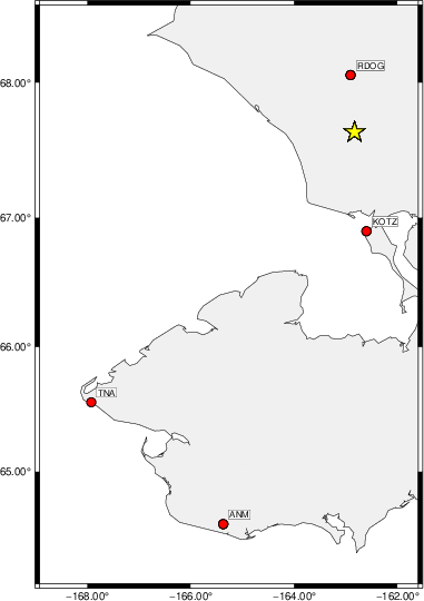
The focal mechanism was determined using broadband seismic waveforms. The location of the event (star) and the stations used for (red) the waveform inversion are shown in the next figure.

Location of broadband stations used for waveform inversion

The program wvfgrd96 was used with good traces observed at short distance to determine the focal mechanism, depth and seismic moment. This technique requires a high quality signal and well determined velocity model for the Green's functions. To the extent that these are the quality data, this type of mechanism should be preferred over the radiation pattern technique which requires the separate step of defining the pressure and tension quadrants and the correct strike.

The observed and predicted traces are filtered using the following gsac commands:

cut o DIST/3.3 -30 o DIST/3.3 +70
rtr
taper w 0.1
hp c 0.03 n 3 
lp c 0.10 n 3 

           DEPTH  STK   DIP  RAKE   MW    FIT
WVFGRD96    1.0   155    90     0   3.74 0.1740
WVFGRD96    2.0   155    90     5   3.92 0.2762
WVFGRD96    3.0   155    90     0   3.99 0.3263
WVFGRD96    4.0   335    85    10   4.06 0.3684
WVFGRD96    5.0   340    85    15   4.08 0.4058
WVFGRD96    6.0   340    85    15   4.13 0.4398
WVFGRD96    7.0   345    80    15   4.15 0.4721
WVFGRD96    8.0   345    80    20   4.21 0.5038
WVFGRD96    9.0   350    80    20   4.23 0.5219
WVFGRD96   10.0   350    80    20   4.25 0.5350
WVFGRD96   11.0   350    80    25   4.29 0.5430
WVFGRD96   12.0   350    80    25   4.30 0.5463
WVFGRD96   13.0   350    80    25   4.32 0.5455
WVFGRD96   14.0   350    80    20   4.33 0.5416
WVFGRD96   15.0   350    80    20   4.34 0.5358
WVFGRD96   16.0   165    75    -5   4.35 0.5333
WVFGRD96   17.0   165    75     0   4.36 0.5271
WVFGRD96   18.0   165    80    10   4.38 0.5210
WVFGRD96   19.0   165    80    15   4.40 0.5151
WVFGRD96   20.0   165    80    15   4.40 0.5102
WVFGRD96   21.0   165    85    25   4.43 0.5062
WVFGRD96   22.0   165    85    30   4.46 0.5021
WVFGRD96   23.0   165    85    30   4.46 0.4968
WVFGRD96   24.0   170    75    30   4.46 0.4921
WVFGRD96   25.0   170    75    30   4.47 0.4878
WVFGRD96   26.0   170    75    25   4.45 0.4837
WVFGRD96   27.0   170    75    25   4.46 0.4786
WVFGRD96   28.0   170    75    25   4.46 0.4736
WVFGRD96   29.0   170    70    25   4.47 0.4680

The best solution is

WVFGRD96   12.0   350    80    25   4.30 0.5463

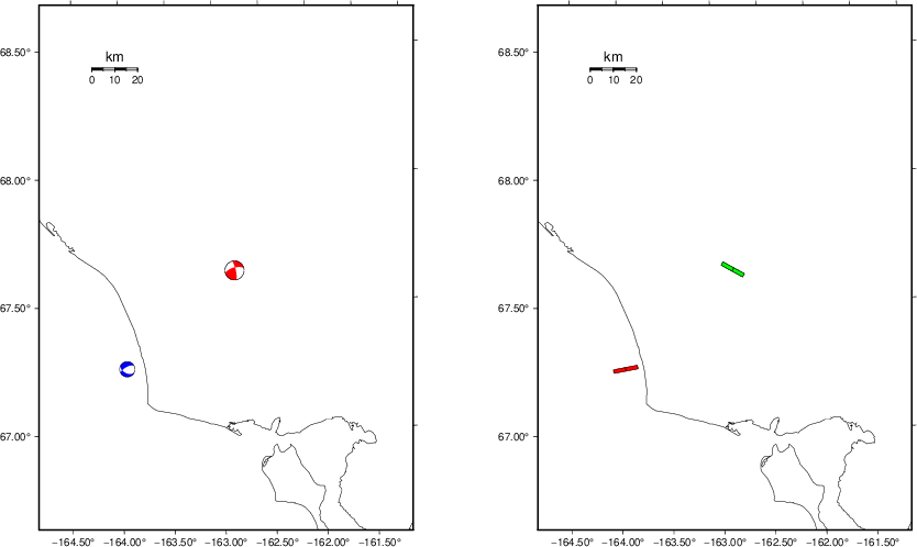
The mechanism corresponding to the best fit is

Figure 1. Waveform inversion focal mechanism

The best fit as a function of depth is given in the following figure:

Figure 2. Depth sensitivity for waveform mechanism

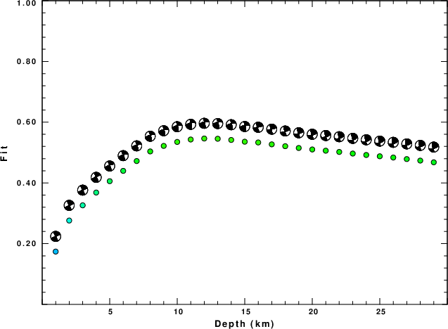
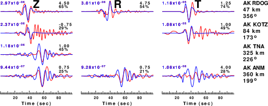
The comparison of the observed and predicted waveforms is given in the next figure. The red traces are the observed and the blue are the predicted. Each observed-predicted component is plotted to the same scale and peak amplitudes are indicated by the numbers to the left of each trace. A pair of numbers is given in black at the right of each predicted traces. The upper number it the time shift required for maximum correlation between the observed and predicted traces. This time shift is required because the synthetics are not computed at exactly the same distance as the observed, the velocity model used in the predictions may not be perfect and the epicentral parameters may be be off. A positive time shift indicates that the prediction is too fast and should be delayed to match the observed trace (shift to the right in this figure). A negative value indicates that the prediction is too slow. The lower number gives the percentage of variance reduction to characterize the individual goodness of fit (100% indicates a perfect fit).

The bandpass filter used in the processing and for the display was

cut o DIST/3.3 -30 o DIST/3.3 +70
rtr
taper w 0.1
hp c 0.03 n 3 
lp c 0.10 n 3 

Figure 3. Waveform comparison for selected depth. Red: observed; Blue - predicted. The time shift with respect to the model prediction is indicated. The percent of fit is also indicated. The time scale is relative to the first trace sample.

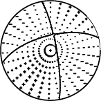
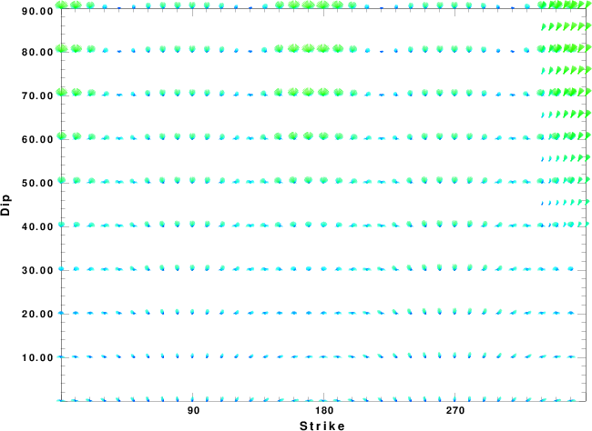
Focal mechanism sensitivity at the preferred depth. The red color indicates a very good fit to the waveforms. Each solution is plotted as a vector at a given value of strike and dip with the angle of the vector representing the rake angle, measured, with respect to the upward vertical (N) in the figure.

A check on the assumed source location is possible by looking at the time shifts between the observed and predicted traces. The time shifts for waveform matching arise for several reasons:

• The origin time and epicentral distance are incorrect
• The velocity model used for the inversion is incorrect
• The velocity model used to define the P-arrival time is not the same as the velocity model used for the waveform inversion (assuming that the initial trace alignment is based on the P arrival time)

 Time_shift = A + B cos Azimuth + C Sin Azimuth

The time shifts for this inversion lead to the next figure:

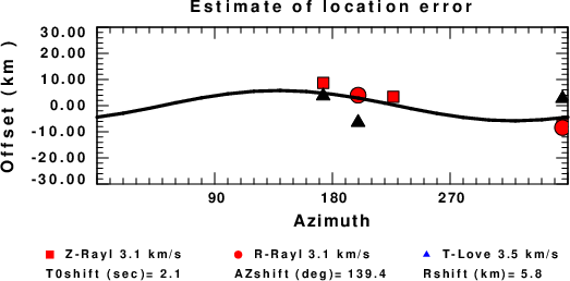
The derived shift in origin time and epicentral coordinates are given at the bottom of the figure.

Velocity Model

The WUS.model used for the waveform synthetic seismograms and for the surface wave eigenfunctions and dispersion is as follows (The format is in the model96 format of Computer Programs in Seismology).

MODEL.01
Model after     8 iterations
ISOTROPIC
KGS
FLAT EARTH
1-D
CONSTANT VELOCITY
LINE08
LINE09
LINE10
LINE11
      H(KM)   VP(KM/S)   VS(KM/S) RHO(GM/CC)         QP         QS       ETAP       ETAS      FREFP      FREFS
     1.9000     3.4065     2.0089     2.2150  0.302E-02  0.679E-02   0.00       0.00       1.00       1.00    
     6.1000     5.5445     3.2953     2.6089  0.349E-02  0.784E-02   0.00       0.00       1.00       1.00    
    13.0000     6.2708     3.7396     2.7812  0.212E-02  0.476E-02   0.00       0.00       1.00       1.00    
    19.0000     6.4075     3.7680     2.8223  0.111E-02  0.249E-02   0.00       0.00       1.00       1.00    
     0.0000     7.9000     4.6200     3.2760  0.164E-10  0.370E-10   0.00       0.00       1.00       1.00