Location
Location ANSS
The ANSS event ID is nc72592670 and the event page is at
https://earthquake.usgs.gov/earthquakes/eventpage/nc72592670/executive.
2016/02/16 23:04:26 37.202 -118.403 15.1 4.77 California
Focal Mechanism
 USGS/SLU Moment Tensor Solution
 ENS  2016/02/16 23:04:26:0  37.20 -118.40  15.1 4.8 California

 Stations used:
   BK.CMB BK.HAST BK.HELL BK.JRSC BK.KCC BK.MHC BK.PACP BK.PKD
   BK.SAO BK.SCZ BK.WENL CI.ADO CI.ARV CI.BAK CI.BCW CI.CCC
   CI.CHF CI.CWC CI.DEC CI.DJJ CI.EDW2 CI.FOX2 CI.FUR CI.GRA
   CI.GSC CI.HEC CI.ISA CI.LMR2 CI.LPC CI.LRL CI.MLAC CI.MOP
   CI.MPM CI.MTP CI.MWC CI.OAT CI.OSI CI.PASC CI.RRX CI.SBC
   CI.SLA CI.SPG2 CI.TFT CI.TUQ CI.VCS CI.VES CI.VOG CI.VTV
   CI.WAS2 CI.WCS2 CI.WLH2 CI.WOR IM.NV31 LB.TPH NC.BBGB
   NC.MCB NC.MDY NC.MINS NC.MLI NC.MMLB NN.BEK NN.CMK6 NN.CTC
   NN.DSP NN.EMB NN.GWY NN.LCH NN.LHV NN.MPK NN.OUT1 NN.PAH
   NN.PNT NN.PRN NN.Q09A NN.QSM NN.REDF NN.RUB NN.RYN NN.S11A
   NN.SHP NN.UNVG NN.VCN NN.WDEM NN.WTNK NN.YER NP.ELK NP.KIR
   NP.MCD NP.MOD NP.PLA SN.HEL TA.R11A US.TPNV

 Filtering commands used:
   cut o DIST/3.3 -30 o DIST/3.3 +70
   rtr
   taper w 0.1
   hp c 0.03 n 3
   lp c 0.06 n 3

 Best Fitting Double Couple
  Mo = 1.41e+23 dyne-cm
  Mw = 4.70
  Z  = 18 km
  Plane   Strike  Dip  Rake
   NP1       35    85    15
   NP2      304    75   175
  Principal Axes:
   Axis    Value   Plunge  Azimuth
    T   1.41e+23     14     260
    N   0.00e+00     74      53
    P  -1.41e+23      7     168

 Moment Tensor: (dyne-cm)
    Component   Value
       Mxx    -1.30e+23
       Mxy     4.95e+22
       Mxz     1.09e+22
       Myy     1.23e+23
       Myz    -3.63e+22
       Mzz     6.35e+21


                     --------------
                 ----------------------
              -------------------------###
             -------------------------#####
           --------------------------########
          ######--------------------##########
         ############--------------############
        #################---------##############
        ####################-----###############
       ##########################################
       #######################---################
       ##   #################-------#############
       ## T ################----------###########
        #   ##############--------------########
        #################-----------------######
         ##############--------------------####
          ############----------------------##
           ##########------------------------
             ######------------------------
              ###-------------------------
                 -------------   ------
                     --------- P --


 Global CMT Convention Moment Tensor:
      R          T          P
  6.35e+21   1.09e+22   3.63e+22
  1.09e+22  -1.30e+23  -4.95e+22
  3.63e+22  -4.95e+22   1.23e+23


Details of the solution is found at

http://www.eas.slu.edu/eqc/eqc_mt/MECH.NA/20160216230426/index.html
|
Preferred Solution
The preferred solution from an analysis of the surface-wave spectral amplitude radiation pattern, waveform inversion or first motion observations is
      STK = 35
      DIP = 85
     RAKE = 15
       MW = 4.70
       HS = 18.0
The NDK file is 20160216230426.ndk
The waveform inversion is preferred.
Moment Tensor Comparison
The following compares this source inversion to those provided by others. The purpose is to look for major differences and also to note slight differences that might be inherent to the processing procedure. For completeness the USGS/SLU solution is repeated from above.
| SLU |
USGSMT |
UCB |
USGSW |
UNR |
 USGS/SLU Moment Tensor Solution
 ENS  2016/02/16 23:04:26:0  37.20 -118.40  15.1 4.8 California

 Stations used:
   BK.CMB BK.HAST BK.HELL BK.JRSC BK.KCC BK.MHC BK.PACP BK.PKD
   BK.SAO BK.SCZ BK.WENL CI.ADO CI.ARV CI.BAK CI.BCW CI.CCC
   CI.CHF CI.CWC CI.DEC CI.DJJ CI.EDW2 CI.FOX2 CI.FUR CI.GRA
   CI.GSC CI.HEC CI.ISA CI.LMR2 CI.LPC CI.LRL CI.MLAC CI.MOP
   CI.MPM CI.MTP CI.MWC CI.OAT CI.OSI CI.PASC CI.RRX CI.SBC
   CI.SLA CI.SPG2 CI.TFT CI.TUQ CI.VCS CI.VES CI.VOG CI.VTV
   CI.WAS2 CI.WCS2 CI.WLH2 CI.WOR IM.NV31 LB.TPH NC.BBGB
   NC.MCB NC.MDY NC.MINS NC.MLI NC.MMLB NN.BEK NN.CMK6 NN.CTC
   NN.DSP NN.EMB NN.GWY NN.LCH NN.LHV NN.MPK NN.OUT1 NN.PAH
   NN.PNT NN.PRN NN.Q09A NN.QSM NN.REDF NN.RUB NN.RYN NN.S11A
   NN.SHP NN.UNVG NN.VCN NN.WDEM NN.WTNK NN.YER NP.ELK NP.KIR
   NP.MCD NP.MOD NP.PLA SN.HEL TA.R11A US.TPNV

 Filtering commands used:
   cut o DIST/3.3 -30 o DIST/3.3 +70
   rtr
   taper w 0.1
   hp c 0.03 n 3
   lp c 0.06 n 3

 Best Fitting Double Couple
  Mo = 1.41e+23 dyne-cm
  Mw = 4.70
  Z  = 18 km
  Plane   Strike  Dip  Rake
   NP1       35    85    15
   NP2      304    75   175
  Principal Axes:
   Axis    Value   Plunge  Azimuth
    T   1.41e+23     14     260
    N   0.00e+00     74      53
    P  -1.41e+23      7     168

 Moment Tensor: (dyne-cm)
    Component   Value
       Mxx    -1.30e+23
       Mxy     4.95e+22
       Mxz     1.09e+22
       Myy     1.23e+23
       Myz    -3.63e+22
       Mzz     6.35e+21


                     --------------
                 ----------------------
              -------------------------###
             -------------------------#####
           --------------------------########
          ######--------------------##########
         ############--------------############
        #################---------##############
        ####################-----###############
       ##########################################
       #######################---################
       ##   #################-------#############
       ## T ################----------###########
        #   ##############--------------########
        #################-----------------######
         ##############--------------------####
          ############----------------------##
           ##########------------------------
             ######------------------------
              ###-------------------------
                 -------------   ------
                     --------- P --


 Global CMT Convention Moment Tensor:
      R          T          P
  6.35e+21   1.09e+22   3.63e+22
  1.09e+22  -1.30e+23  -4.95e+22
  3.63e+22  -4.95e+22   1.23e+23


Details of the solution is found at

http://www.eas.slu.edu/eqc/eqc_mt/MECH.NA/20160216230426/index.html
|
Regional Moment Tensor (Mwr)
Moment	1.818e+16 N-m
Magnitude	4.77
Depth	24.0 km
Percent DC	100%
Half Duration	–
Catalog	US (us200050nt)
Data Source	NC1
Contributor	US3
Nodal Planes
Plane	Strike	Dip	Rake
NP1	306	81	-179
NP2	216	89	-9
Principal Axes
Axis	Value	Plunge	Azimuth
T	1.819	5	261
N	-0.002	81	27
P	-1.817	7	171

|
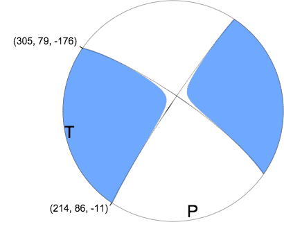
TMTS
Moment	1.757e+16 N-m
Magnitude	4.76
Depth	18.0 km
Percent DC	96%
Half Duration	–
Catalog	NC (nc72592670)
Data Source	NC1
Contributor	NC1
Nodal Planes
Plane	Strike	Dip	Rake
NP1	305	79	-176
NP2	214	86	-11
Principal Axes
Axis	Value	Plunge	Azimuth
T	1.774	5	260
N	-0.034	79	13
P	-1.739	10	169
|
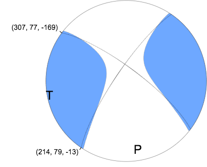
W-phase Moment Tensor (Mww)
Moment	1.859e+16 N-m
Magnitude	4.78
Depth	19.5 km
Percent DC	75%
Half Duration	–
Catalog	US (us200050nt)
Data Source	US3
Contributor	US3
Nodal Planes
Plane	Strike	Dip	Rake
NP1	307	77	-169
NP2	214	79	-13
Principal Axes
Axis	Value	Plunge	Azimuth
T	1.969	1	261
N	-0.244	73	355
P	-1.725	17	170
|
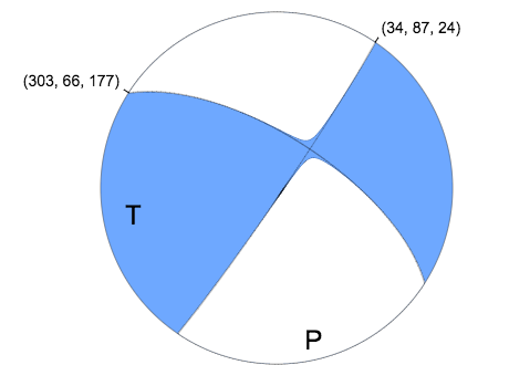
Mw
Moment	1.164e+16 N-m
Magnitude	4.64
Depth	12.0 km
Percent DC	99%
Half Duration	–
Catalog	NN (nn00531804)
Data Source	NN2
Contributor	NN2
Nodal Planes
Plane	Strike	Dip	Rake
NP1	303	66	177
NP2	34	87	24
Principal Axes
Axis	Value	Plunge	Azimuth
T	1.156	19	261
N	0.006	66	40
P	-1.172	14	166
|
Magnitudes
Given the availability of digital waveforms for determination of the moment tensor, this section documents the added processing leading to mLg, if appropriate to the region, and ML by application of the respective IASPEI formulae. As a research study, the linear distance term of the IASPEI formula
for ML is adjusted to remove a linear distance trend in residuals to give a regionally defined ML. The defined ML uses horizontal component recordings, but the same procedure is applied to the vertical components since there may be some interest in vertical component ground motions. Residual plots versus distance may indicate interesting features of ground motion scaling in some distance ranges. A residual plot of the regionalized magnitude is given as a function of distance and azimuth, since data sets may transcend different wave propagation provinces.
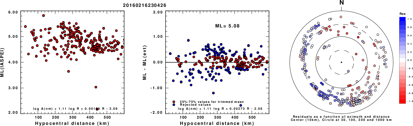
ML Magnitude
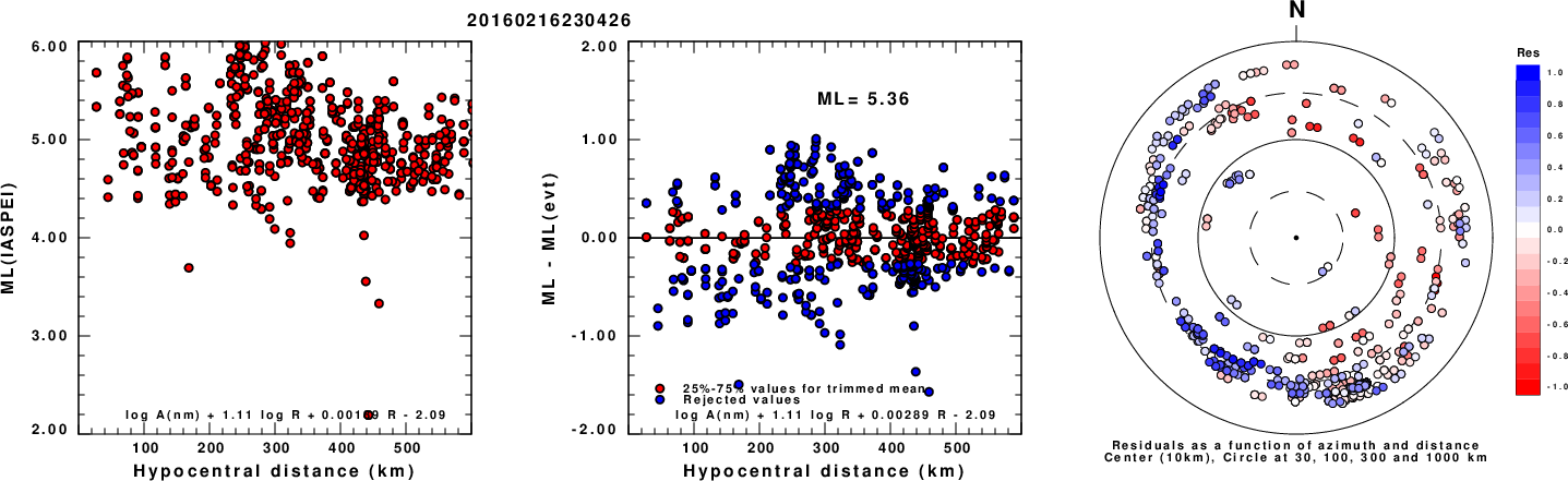
Left: ML computed using the IASPEI formula for Horizontal components. Center: ML residuals computed using a modified IASPEI formula that accounts for path specific attenuation; the values used for the trimmed mean are indicated. The ML relation used for each figure is given at the bottom of each plot.
Right: Residuals from new relation as a function of distance and azimuth.
Left: ML computed using the IASPEI formula for Vertical components (research). Center: ML residuals computed using a modified IASPEI formula that accounts for path specific attenuation; the values used for the trimmed mean are indicated. The ML relation used for each figure is given at the bottom of each plot.
Right: Residuals from new relation as a function of distance and azimuth.
Context
The left panel of the next figure presents the focal mechanism for this earthquake (red) in the context of other nearby events (blue) in the SLU Moment Tensor Catalog. The right panel shows the inferred direction of maximum compressive stress and the type of faulting (green is strike-slip, red is normal, blue is thrust; oblique is shown by a combination of colors). Thus context plot is useful for assessing the appropriateness of the moment tensor of this event.
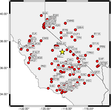
Waveform Inversion using wvfgrd96
The focal mechanism was determined using broadband seismic waveforms. The location of the event (star) and the
stations used for (red) the waveform inversion are shown in the next figure.
|
|
Location of broadband stations used for waveform inversion
|
The program wvfgrd96 was used with good traces observed at short distance to determine the focal mechanism, depth and seismic moment. This technique requires a high quality signal and well determined velocity model for the Green's functions. To the extent that these are the quality data, this type of mechanism should be preferred over the radiation pattern technique which requires the separate step of defining the pressure and tension quadrants and the correct strike.
The observed and predicted traces are filtered using the following gsac commands:
cut o DIST/3.3 -30 o DIST/3.3 +70
rtr
taper w 0.1
hp c 0.03 n 3
lp c 0.06 n 3
The results of this grid search are as follow:
           DEPTH  STK   DIP  RAKE   MW    FIT
WVFGRD96    1.0   215    90     0   4.23 0.3026
WVFGRD96    2.0   215    90     0   4.34 0.3967
WVFGRD96    3.0   215    90   -10   4.39 0.4384
WVFGRD96    4.0   215    90   -20   4.44 0.4684
WVFGRD96    5.0   215    90   -20   4.47 0.4956
WVFGRD96    6.0   215    85   -20   4.50 0.5232
WVFGRD96    7.0   215    85   -20   4.53 0.5534
WVFGRD96    8.0   215    85   -25   4.57 0.5839
WVFGRD96    9.0   215    90   -25   4.59 0.6086
WVFGRD96   10.0   215    90   -20   4.60 0.6310
WVFGRD96   11.0   215    90   -20   4.62 0.6516
WVFGRD96   12.0   215    90   -20   4.63 0.6687
WVFGRD96   13.0    35    85    20   4.65 0.6828
WVFGRD96   14.0    35    85    15   4.66 0.6946
WVFGRD96   15.0    35    85    15   4.67 0.7044
WVFGRD96   16.0    35    85    15   4.68 0.7109
WVFGRD96   17.0    35    85    15   4.69 0.7146
WVFGRD96   18.0    35    85    15   4.70 0.7157
WVFGRD96   19.0   215    90   -15   4.71 0.7129
WVFGRD96   20.0   215    90   -15   4.71 0.7103
WVFGRD96   21.0    35    85    15   4.72 0.7078
WVFGRD96   22.0    35    85    15   4.73 0.7022
WVFGRD96   23.0    35    85    15   4.74 0.6956
WVFGRD96   24.0   215    90   -15   4.74 0.6878
WVFGRD96   25.0    35    85    15   4.75 0.6800
WVFGRD96   26.0    35    90    15   4.75 0.6715
WVFGRD96   27.0    35    90    15   4.76 0.6627
WVFGRD96   28.0    35    90    15   4.77 0.6535
WVFGRD96   29.0    35    90    10   4.77 0.6441
The best solution is
WVFGRD96 18.0 35 85 15 4.70 0.7157
The mechanism corresponding to the best fit is
|
|
Figure 1. Waveform inversion focal mechanism
|
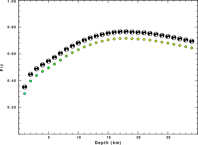
The best fit as a function of depth is given in the following figure:
|
|
Figure 2. Depth sensitivity for waveform mechanism
|
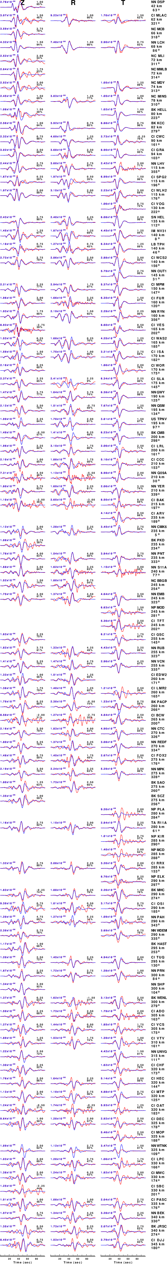
The comparison of the observed and predicted waveforms is given in the next figure. The red traces are the observed and the blue are the predicted.
Each observed-predicted component is plotted to the same scale and peak amplitudes are indicated by the numbers to the left of each trace. A pair of numbers is given in black at the right of each predicted traces. The upper number it the time shift required for maximum correlation between the observed and predicted traces. This time shift is required because the synthetics are not computed at exactly the same distance as the observed, the velocity model used in the predictions may not be perfect and the epicentral parameters may be be off.
A positive time shift indicates that the prediction is too fast and should be delayed to match the observed trace (shift to the right in this figure). A negative value indicates that the prediction is too slow. The lower number gives the percentage of variance reduction to characterize the individual goodness of fit (100% indicates a perfect fit).
The bandpass filter used in the processing and for the display was
cut o DIST/3.3 -30 o DIST/3.3 +70
rtr
taper w 0.1
hp c 0.03 n 3
lp c 0.06 n 3
|
|
Figure 3. Waveform comparison for selected depth. Red: observed; Blue - predicted. The time shift with respect to the model prediction is indicated. The percent of fit is also indicated. The time scale is relative to the first trace sample.
|
|
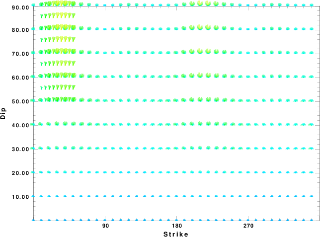
|
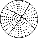
Focal mechanism sensitivity at the preferred depth. The red color indicates a very good fit to the waveforms.
Each solution is plotted as a vector at a given value of strike and dip with the angle of the vector representing the rake angle, measured, with respect to the upward vertical (N) in the figure.
|
A check on the assumed source location is possible by looking at the time shifts between the observed and predicted traces. The time shifts for waveform matching arise for several reasons:
- The origin time and epicentral distance are incorrect
- The velocity model used for the inversion is incorrect
- The velocity model used to define the P-arrival time is not the
same as the velocity model used for the waveform inversion
(assuming that the initial trace alignment is based on the
P arrival time)
Assuming only a mislocation, the time shifts are fit to a functional form:
Time_shift = A + B cos Azimuth + C Sin Azimuth
The time shifts for this inversion lead to the next figure:
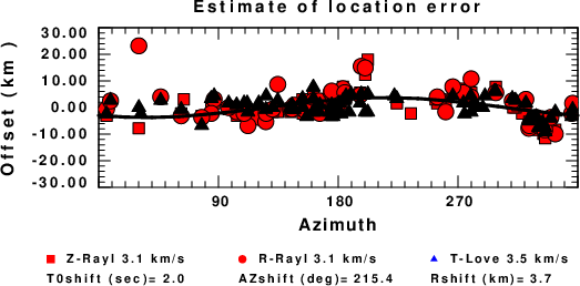
The derived shift in origin time and epicentral coordinates are given at the bottom of the figure.
Velocity Model
The WUS.model used for the waveform synthetic seismograms and for the surface wave eigenfunctions and dispersion is as follows
(The format is in the model96 format of Computer Programs in Seismology).
MODEL.01
Model after     8 iterations
ISOTROPIC
KGS
FLAT EARTH
1-D
CONSTANT VELOCITY
LINE08
LINE09
LINE10
LINE11
      H(KM)   VP(KM/S)   VS(KM/S) RHO(GM/CC)         QP         QS       ETAP       ETAS      FREFP      FREFS
     1.9000     3.4065     2.0089     2.2150  0.302E-02  0.679E-02   0.00       0.00       1.00       1.00
     6.1000     5.5445     3.2953     2.6089  0.349E-02  0.784E-02   0.00       0.00       1.00       1.00
    13.0000     6.2708     3.7396     2.7812  0.212E-02  0.476E-02   0.00       0.00       1.00       1.00
    19.0000     6.4075     3.7680     2.8223  0.111E-02  0.249E-02   0.00       0.00       1.00       1.00
     0.0000     7.9000     4.6200     3.2760  0.164E-10  0.370E-10   0.00       0.00       1.00       1.00
Last Changed Fri Apr 26 01:59:20 PM CDT 2024
