Location
Location ANSS
The ANSS event ID is us20004zy8 and the event page is at
https://earthquake.usgs.gov/earthquakes/eventpage/us20004zy8/executive.
2016/02/13 17:07:06 36.490 -98.709 8.3 5.1 Oklahoma
Focal Mechanism
 USGS/SLU Moment Tensor Solution
 ENS  2016/02/13 17:07:06:0  36.49  -98.71   8.3 5.1 Oklahoma

 Stations used:
   AG.HHAR GS.KAN01 GS.KAN05 GS.KAN06 GS.KAN08 GS.KAN10
   GS.KAN11 GS.KAN12 GS.KAN13 GS.KAN14 GS.KAN16 GS.KAN17
   GS.OK025 GS.OK029 GS.OK030 GS.OK031 GS.OK032 GS.OK033
   GS.OK034 GS.OK035 N4.N33B N4.R32B N4.S39B N4.T35B N4.U38B
   OK.BCOK OK.BLOK OK.CCOK OK.CHOK OK.CROK OK.FNO OK.GORE
   OK.OKCFA OK.QUOK OK.RLOK OK.U32A OK.W35A OK.X34A OK.X37A
   TA.ABTX TA.BGNE TA.KSCO TA.MSTX TA.T25A TA.TUL1 TA.U40A
   TA.W39A US.AMTX US.CBKS US.KSU1 US.MIAR US.WMOK

 Filtering commands used:
   cut o DIST/3.3 -30 o DIST/3.3 +70
   rtr
   taper w 0.1
   hp c 0.03 n 3
   lp c 0.07 n 3

 Best Fitting Double Couple
  Mo = 3.98e+23 dyne-cm
  Mw = 5.00
  Z  = 9 km
  Plane   Strike  Dip  Rake
   NP1       42    80   -170
   NP2      310    80   -10
  Principal Axes:
   Axis    Value   Plunge  Azimuth
    T   3.98e+23      0     176
    N   0.00e+00     76      85
    P  -3.98e+23     14     266

 Moment Tensor: (dyne-cm)
    Component   Value
       Mxx     3.94e+23
       Mxy    -5.54e+22
       Mxz     6.00e+21
       Myy    -3.70e+23
       Myz     9.39e+22
       Mzz    -2.36e+22


                     ##############
                 ######################
              ############################
             ############################--
           ----#########################-----
          --------#####################-------
         ------------#################---------
        ----------------############------------
        ------------------#########-------------
       ----------------------#####---------------
       -   --------------------#-----------------
       - P --------------------##----------------
       -   ------------------######--------------
        -------------------##########-----------
        -----------------##############---------
         --------------#################-------
          -----------#####################----
           --------########################--
             ----##########################
              ############################
                 ###########   ########
                     ####### T ####


 Global CMT Convention Moment Tensor:
      R          T          P
 -2.36e+22   6.00e+21  -9.39e+22
  6.00e+21   3.94e+23   5.54e+22
 -9.39e+22   5.54e+22  -3.70e+23


Details of the solution is found at

http://www.eas.slu.edu/eqc/eqc_mt/MECH.NA/20160213170706/index.html
|
Preferred Solution
The preferred solution from an analysis of the surface-wave spectral amplitude radiation pattern, waveform inversion or first motion observations is
      STK = 310
      DIP = 80
     RAKE = -10
       MW = 5.00
       HS = 9.0
The NDK file is 20160213170706.ndk
The waveform inversion is preferred.
Moment Tensor Comparison
The following compares this source inversion to those provided by others. The purpose is to look for major differences and also to note slight differences that might be inherent to the processing procedure. For completeness the USGS/SLU solution is repeated from above.
| SLU |
USGSMT |
USGSW |
 USGS/SLU Moment Tensor Solution
 ENS  2016/02/13 17:07:06:0  36.49  -98.71   8.3 5.1 Oklahoma

 Stations used:
   AG.HHAR GS.KAN01 GS.KAN05 GS.KAN06 GS.KAN08 GS.KAN10
   GS.KAN11 GS.KAN12 GS.KAN13 GS.KAN14 GS.KAN16 GS.KAN17
   GS.OK025 GS.OK029 GS.OK030 GS.OK031 GS.OK032 GS.OK033
   GS.OK034 GS.OK035 N4.N33B N4.R32B N4.S39B N4.T35B N4.U38B
   OK.BCOK OK.BLOK OK.CCOK OK.CHOK OK.CROK OK.FNO OK.GORE
   OK.OKCFA OK.QUOK OK.RLOK OK.U32A OK.W35A OK.X34A OK.X37A
   TA.ABTX TA.BGNE TA.KSCO TA.MSTX TA.T25A TA.TUL1 TA.U40A
   TA.W39A US.AMTX US.CBKS US.KSU1 US.MIAR US.WMOK

 Filtering commands used:
   cut o DIST/3.3 -30 o DIST/3.3 +70
   rtr
   taper w 0.1
   hp c 0.03 n 3
   lp c 0.07 n 3

 Best Fitting Double Couple
  Mo = 3.98e+23 dyne-cm
  Mw = 5.00
  Z  = 9 km
  Plane   Strike  Dip  Rake
   NP1       42    80   -170
   NP2      310    80   -10
  Principal Axes:
   Axis    Value   Plunge  Azimuth
    T   3.98e+23      0     176
    N   0.00e+00     76      85
    P  -3.98e+23     14     266

 Moment Tensor: (dyne-cm)
    Component   Value
       Mxx     3.94e+23
       Mxy    -5.54e+22
       Mxz     6.00e+21
       Myy    -3.70e+23
       Myz     9.39e+22
       Mzz    -2.36e+22


                     ##############
                 ######################
              ############################
             ############################--
           ----#########################-----
          --------#####################-------
         ------------#################---------
        ----------------############------------
        ------------------#########-------------
       ----------------------#####---------------
       -   --------------------#-----------------
       - P --------------------##----------------
       -   ------------------######--------------
        -------------------##########-----------
        -----------------##############---------
         --------------#################-------
          -----------#####################----
           --------########################--
             ----##########################
              ############################
                 ###########   ########
                     ####### T ####


 Global CMT Convention Moment Tensor:
      R          T          P
 -2.36e+22   6.00e+21  -9.39e+22
  6.00e+21   3.94e+23   5.54e+22
 -9.39e+22   5.54e+22  -3.70e+23


Details of the solution is found at

http://www.eas.slu.edu/eqc/eqc_mt/MECH.NA/20160213170706/index.html
|
Regional Moment Tensor (Mwr)
Moment 4.988e+16 N-m
Magnitude 5.07
Depth 8.0 km
Percent DC 90%
Half Duration –
Catalog US (us20004zy8)
Data Source US1
Contributor US1
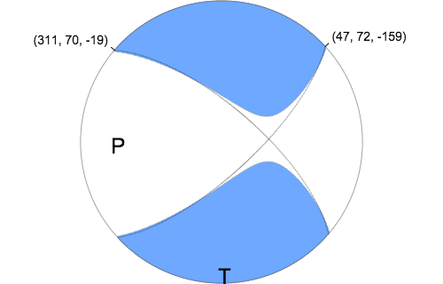
Nodal Planes
Plane Strike Dip Rake
NP1 311 70 -19
NP2 47 72 -159
Principal Axes
Axis Value Plunge Azimuth
T 5.112 1 179
N -0.259 62 86
P -4.853 27 269
|
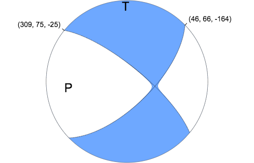
W-phase Moment Tensor (Mww)
Moment	6.159e+16 N-m
Magnitude	5.13
Depth	11.5 km
Percent DC	99%
Half Duration	–
Catalog	US (us20004zy8)
Data Source	US1
Contributor	US1
Nodal Planes
Plane	Strike	Dip	Rake
NP1	46	66	-164
NP2	309	75	-25
|
Magnitudes
Given the availability of digital waveforms for determination of the moment tensor, this section documents the added processing leading to mLg, if appropriate to the region, and ML by application of the respective IASPEI formulae. As a research study, the linear distance term of the IASPEI formula
for ML is adjusted to remove a linear distance trend in residuals to give a regionally defined ML. The defined ML uses horizontal component recordings, but the same procedure is applied to the vertical components since there may be some interest in vertical component ground motions. Residual plots versus distance may indicate interesting features of ground motion scaling in some distance ranges. A residual plot of the regionalized magnitude is given as a function of distance and azimuth, since data sets may transcend different wave propagation provinces.
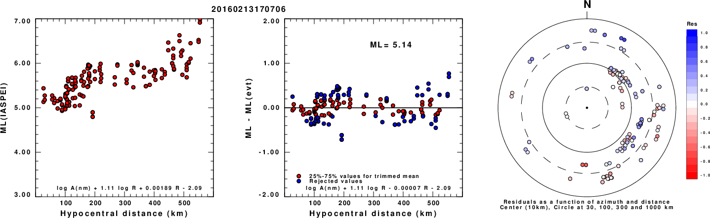
mLg Magnitude
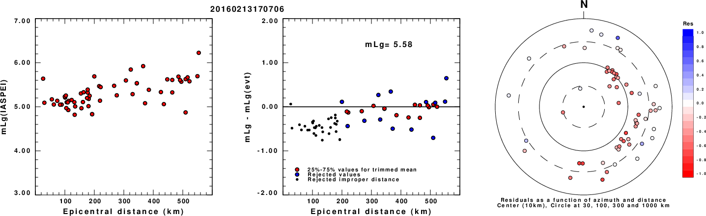
Left: mLg computed using the IASPEI formula. Center: mLg residuals versus epicentral distance ; the values used for the trimmed mean magnitude estimate are indicated.
Right: residuals as a function of distance and azimuth.
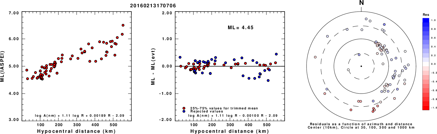
ML Magnitude
Left: ML computed using the IASPEI formula for Horizontal components. Center: ML residuals computed using a modified IASPEI formula that accounts for path specific attenuation; the values used for the trimmed mean are indicated. The ML relation used for each figure is given at the bottom of each plot.
Right: Residuals from new relation as a function of distance and azimuth.
Left: ML computed using the IASPEI formula for Vertical components (research). Center: ML residuals computed using a modified IASPEI formula that accounts for path specific attenuation; the values used for the trimmed mean are indicated. The ML relation used for each figure is given at the bottom of each plot.
Right: Residuals from new relation as a function of distance and azimuth.
Context
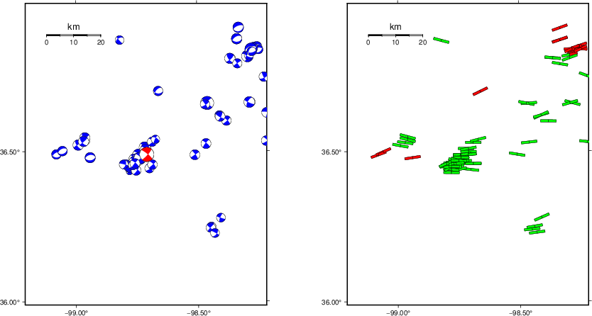
The left panel of the next figure presents the focal mechanism for this earthquake (red) in the context of other nearby events (blue) in the SLU Moment Tensor Catalog. The right panel shows the inferred direction of maximum compressive stress and the type of faulting (green is strike-slip, red is normal, blue is thrust; oblique is shown by a combination of colors). Thus context plot is useful for assessing the appropriateness of the moment tensor of this event.
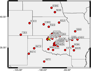
Waveform Inversion using wvfgrd96
The focal mechanism was determined using broadband seismic waveforms. The location of the event (star) and the
stations used for (red) the waveform inversion are shown in the next figure.
|
|
Location of broadband stations used for waveform inversion
|
The program wvfgrd96 was used with good traces observed at short distance to determine the focal mechanism, depth and seismic moment. This technique requires a high quality signal and well determined velocity model for the Green's functions. To the extent that these are the quality data, this type of mechanism should be preferred over the radiation pattern technique which requires the separate step of defining the pressure and tension quadrants and the correct strike.
The observed and predicted traces are filtered using the following gsac commands:
cut o DIST/3.3 -30 o DIST/3.3 +70
rtr
taper w 0.1
hp c 0.03 n 3
lp c 0.07 n 3
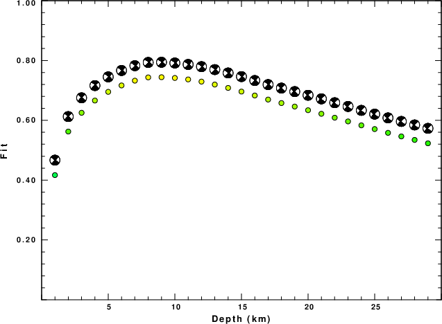
The results of this grid search are as follow:
           DEPTH  STK   DIP  RAKE   MW    FIT
WVFGRD96    1.0   310    85    -5   4.65 0.4169
WVFGRD96    2.0   315    85     5   4.77 0.5625
WVFGRD96    3.0   315    80     5   4.83 0.6253
WVFGRD96    4.0   315    75     5   4.87 0.6662
WVFGRD96    5.0   310    75   -10   4.90 0.6953
WVFGRD96    6.0   310    80   -10   4.93 0.7167
WVFGRD96    7.0   310    80   -10   4.95 0.7327
WVFGRD96    8.0   310    75   -10   4.98 0.7436
WVFGRD96    9.0   310    80   -10   5.00 0.7442
WVFGRD96   10.0   310    80   -10   5.02 0.7417
WVFGRD96   11.0   310    80   -10   5.03 0.7368
WVFGRD96   12.0   310    80   -10   5.04 0.7295
WVFGRD96   13.0   310    80   -10   5.05 0.7197
WVFGRD96   14.0   310    80   -10   5.06 0.7084
WVFGRD96   15.0   310    80   -10   5.07 0.6962
WVFGRD96   16.0   310    80    -5   5.08 0.6831
WVFGRD96   17.0   310    80    -5   5.09 0.6695
WVFGRD96   18.0   135    85   -10   5.09 0.6578
WVFGRD96   19.0   135    85   -10   5.10 0.6461
WVFGRD96   20.0   135    85   -10   5.11 0.6339
WVFGRD96   21.0   130    80   -10   5.12 0.6219
WVFGRD96   22.0   130    80   -10   5.12 0.6089
WVFGRD96   23.0   130    80   -10   5.13 0.5964
WVFGRD96   24.0   130    80   -10   5.14 0.5833
WVFGRD96   25.0   130    80   -10   5.14 0.5708
WVFGRD96   26.0   130    80   -10   5.15 0.5582
WVFGRD96   27.0   130    80   -10   5.15 0.5463
WVFGRD96   28.0   130    80   -10   5.16 0.5346
WVFGRD96   29.0   130    80   -10   5.16 0.5232
The best solution is
WVFGRD96 9.0 310 80 -10 5.00 0.7442
The mechanism corresponding to the best fit is
|
|
Figure 1. Waveform inversion focal mechanism
|
The best fit as a function of depth is given in the following figure:
|
|
Figure 2. Depth sensitivity for waveform mechanism
|
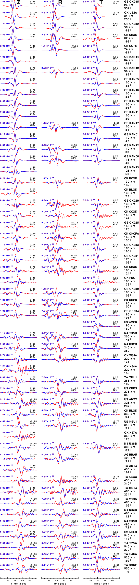
The comparison of the observed and predicted waveforms is given in the next figure. The red traces are the observed and the blue are the predicted.
Each observed-predicted component is plotted to the same scale and peak amplitudes are indicated by the numbers to the left of each trace. A pair of numbers is given in black at the right of each predicted traces. The upper number it the time shift required for maximum correlation between the observed and predicted traces. This time shift is required because the synthetics are not computed at exactly the same distance as the observed, the velocity model used in the predictions may not be perfect and the epicentral parameters may be be off.
A positive time shift indicates that the prediction is too fast and should be delayed to match the observed trace (shift to the right in this figure). A negative value indicates that the prediction is too slow. The lower number gives the percentage of variance reduction to characterize the individual goodness of fit (100% indicates a perfect fit).
The bandpass filter used in the processing and for the display was
cut o DIST/3.3 -30 o DIST/3.3 +70
rtr
taper w 0.1
hp c 0.03 n 3
lp c 0.07 n 3
|
|
Figure 3. Waveform comparison for selected depth. Red: observed; Blue - predicted. The time shift with respect to the model prediction is indicated. The percent of fit is also indicated. The time scale is relative to the first trace sample.
|
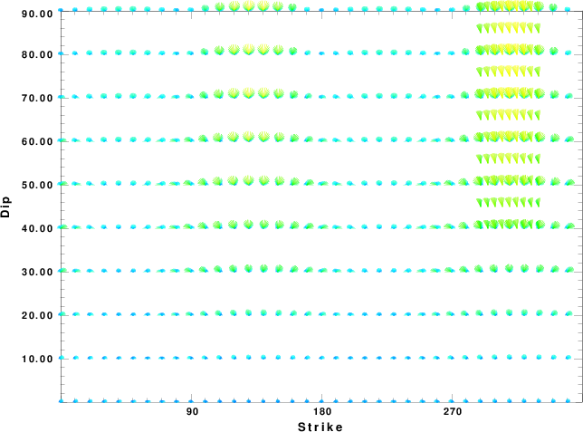
|
|
Focal mechanism sensitivity at the preferred depth. The red color indicates a very good fit to the waveforms.
Each solution is plotted as a vector at a given value of strike and dip with the angle of the vector representing the rake angle, measured, with respect to the upward vertical (N) in the figure.
|
A check on the assumed source location is possible by looking at the time shifts between the observed and predicted traces. The time shifts for waveform matching arise for several reasons:
- The origin time and epicentral distance are incorrect
- The velocity model used for the inversion is incorrect
- The velocity model used to define the P-arrival time is not the
same as the velocity model used for the waveform inversion
(assuming that the initial trace alignment is based on the
P arrival time)
Assuming only a mislocation, the time shifts are fit to a functional form:
Time_shift = A + B cos Azimuth + C Sin Azimuth
The time shifts for this inversion lead to the next figure:
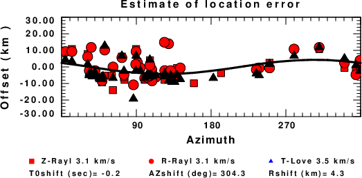
The derived shift in origin time and epicentral coordinates are given at the bottom of the figure.
Velocity Model
The WUS.model used for the waveform synthetic seismograms and for the surface wave eigenfunctions and dispersion is as follows
(The format is in the model96 format of Computer Programs in Seismology).
MODEL.01
Model after     8 iterations
ISOTROPIC
KGS
FLAT EARTH
1-D
CONSTANT VELOCITY
LINE08
LINE09
LINE10
LINE11
      H(KM)   VP(KM/S)   VS(KM/S) RHO(GM/CC)         QP         QS       ETAP       ETAS      FREFP      FREFS
     1.9000     3.4065     2.0089     2.2150  0.302E-02  0.679E-02   0.00       0.00       1.00       1.00
     6.1000     5.5445     3.2953     2.6089  0.349E-02  0.784E-02   0.00       0.00       1.00       1.00
    13.0000     6.2708     3.7396     2.7812  0.212E-02  0.476E-02   0.00       0.00       1.00       1.00
    19.0000     6.4075     3.7680     2.8223  0.111E-02  0.249E-02   0.00       0.00       1.00       1.00
     0.0000     7.9000     4.6200     3.2760  0.164E-10  0.370E-10   0.00       0.00       1.00       1.00
Last Changed Fri Apr 26 01:39:09 PM CDT 2024