Location
Location ANSS
The ANSS event ID is ci37299263 and the event page is at
https://earthquake.usgs.gov/earthquakes/eventpage/ci37299263/executive.
2016/01/24 15:32:16 34.697 -116.239 2.6 4.11 California
Focal Mechanism
 USGS/SLU Moment Tensor Solution
 ENS  2016/01/24 15:32:16:0  34.70 -116.24   2.6 4.1 California

 Stations used:
   AE.W13A AZ.FRD AZ.PFO AZ.RRSP AZ.SMER AZ.SND CI.ADO CI.BAR
   CI.BBR CI.BC3 CI.BEL CI.BFS CI.CCC CI.CGO CI.CHF CI.CWC
   CI.DAN CI.DEC CI.DGR CI.DJJ CI.EDW2 CI.FOX2 CI.FUR CI.GLA
   CI.GMR CI.GRA CI.GSC CI.HEC CI.ISA CI.LMR2 CI.LPC CI.MOP
   CI.MPM CI.MTP CI.MUR CI.MWC CI.NEE2 CI.OSI CI.PASC CI.PMD
   CI.RRX CI.RVR CI.SHO CI.SLA CI.SPG2 CI.TIN CI.TUQ CI.USC
   CI.VCS CI.VTV CI.WCS2 NN.LCH NN.SHP NN.V12A PY.BPH01
   PY.BPH10 YN.GVAR1 YN.JF00 YN.RHIL YN.TR01

 Filtering commands used:
   cut o DIST/3.3 -20 o DIST/3.3 +50
   rtr
   taper w 0.1
   hp c 0.03 n 3
   lp c 0.07 n 3

 Best Fitting Double Couple
  Mo = 1.10e+22 dyne-cm
  Mw = 3.96
  Z  = 11 km
  Plane   Strike  Dip  Rake
   NP1      151    72   154
   NP2      250    65    20
  Principal Axes:
   Axis    Value   Plunge  Azimuth
    T   1.10e+22     31     109
    N   0.00e+00     58     299
    P  -1.10e+22      5     202

 Moment Tensor: (dyne-cm)
    Component   Value
       Mxx    -8.54e+21
       Mxy    -6.23e+21
       Mxz    -7.76e+20
       Myy     5.67e+21
       Myz     4.92e+21
       Mzz     2.87e+21


                     --------------
                 #---------------------
              ####------------------------
             #####-------------------------
           #######---------------------------
          #########---------------------------
         ##########-----------------#######----
        ############-------#####################
        #############--#########################
       ############---###########################
       #########------###########################
       #######---------##########################
       #####------------################   ######
        ##---------------############### T #####
        #------------------#############   #####
         -------------------###################
          -------------------#################
           --------------------##############
             -------------------###########
              -----   ------------########
                 -- P ---------------##
                      -------------


 Global CMT Convention Moment Tensor:
      R          T          P
  2.87e+21  -7.76e+20  -4.92e+21
 -7.76e+20  -8.54e+21   6.23e+21
 -4.92e+21   6.23e+21   5.67e+21


Details of the solution is found at

http://www.eas.slu.edu/eqc/eqc_mt/MECH.NA/20160124153216/index.html
|
Preferred Solution
The preferred solution from an analysis of the surface-wave spectral amplitude radiation pattern, waveform inversion or first motion observations is
      STK = 250
      DIP = 65
     RAKE = 20
       MW = 3.96
       HS = 11.0
The NDK file is 20160124153216.ndk
The waveform inversion is preferred.
Moment Tensor Comparison
The following compares this source inversion to those provided by others. The purpose is to look for major differences and also to note slight differences that might be inherent to the processing procedure. For completeness the USGS/SLU solution is repeated from above.
| SLU |
SCAL |
 USGS/SLU Moment Tensor Solution
 ENS  2016/01/24 15:32:16:0  34.70 -116.24   2.6 4.1 California

 Stations used:
   AE.W13A AZ.FRD AZ.PFO AZ.RRSP AZ.SMER AZ.SND CI.ADO CI.BAR
   CI.BBR CI.BC3 CI.BEL CI.BFS CI.CCC CI.CGO CI.CHF CI.CWC
   CI.DAN CI.DEC CI.DGR CI.DJJ CI.EDW2 CI.FOX2 CI.FUR CI.GLA
   CI.GMR CI.GRA CI.GSC CI.HEC CI.ISA CI.LMR2 CI.LPC CI.MOP
   CI.MPM CI.MTP CI.MUR CI.MWC CI.NEE2 CI.OSI CI.PASC CI.PMD
   CI.RRX CI.RVR CI.SHO CI.SLA CI.SPG2 CI.TIN CI.TUQ CI.USC
   CI.VCS CI.VTV CI.WCS2 NN.LCH NN.SHP NN.V12A PY.BPH01
   PY.BPH10 YN.GVAR1 YN.JF00 YN.RHIL YN.TR01

 Filtering commands used:
   cut o DIST/3.3 -20 o DIST/3.3 +50
   rtr
   taper w 0.1
   hp c 0.03 n 3
   lp c 0.07 n 3

 Best Fitting Double Couple
  Mo = 1.10e+22 dyne-cm
  Mw = 3.96
  Z  = 11 km
  Plane   Strike  Dip  Rake
   NP1      151    72   154
   NP2      250    65    20
  Principal Axes:
   Axis    Value   Plunge  Azimuth
    T   1.10e+22     31     109
    N   0.00e+00     58     299
    P  -1.10e+22      5     202

 Moment Tensor: (dyne-cm)
    Component   Value
       Mxx    -8.54e+21
       Mxy    -6.23e+21
       Mxz    -7.76e+20
       Myy     5.67e+21
       Myz     4.92e+21
       Mzz     2.87e+21


                     --------------
                 #---------------------
              ####------------------------
             #####-------------------------
           #######---------------------------
          #########---------------------------
         ##########-----------------#######----
        ############-------#####################
        #############--#########################
       ############---###########################
       #########------###########################
       #######---------##########################
       #####------------################   ######
        ##---------------############### T #####
        #------------------#############   #####
         -------------------###################
          -------------------#################
           --------------------##############
             -------------------###########
              -----   ------------########
                 -- P ---------------##
                      -------------


 Global CMT Convention Moment Tensor:
      R          T          P
  2.87e+21  -7.76e+20  -4.92e+21
 -7.76e+20  -8.54e+21   6.23e+21
 -4.92e+21   6.23e+21   5.67e+21


Details of the solution is found at

http://www.eas.slu.edu/eqc/eqc_mt/MECH.NA/20160124153216/index.html
|
Scientific - Focal Mechanism
Data Source CI1
Catalog CI (ci37299263)
Data Source CI1
Contributor CI1
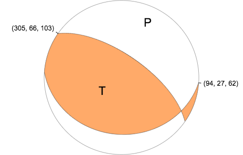
Nodal Planes
Plane Strike Dip Rake
NP1 305 66 103
NP2 94 27 62
TMTS
Moment	1.790e+15 N-m
Magnitude	4.10
Depth	5.0 km
Percent DC	93%
Half Duration	–
Catalog	CI (ci37299263)
Data Source	CI1
Contributor	CI1
Nodal Planes
Plane	Strike	Dip	Rake
NP1	191	50	-104
NP2	32	42	-74
Principal Axes
Axis	Value	Plunge	Azimuth
T	1.757	4	291
N	0.064	10	200
P	-1.822	79	43

|
|
Magnitudes
Given the availability of digital waveforms for determination of the moment tensor, this section documents the added processing leading to mLg, if appropriate to the region, and ML by application of the respective IASPEI formulae. As a research study, the linear distance term of the IASPEI formula
for ML is adjusted to remove a linear distance trend in residuals to give a regionally defined ML. The defined ML uses horizontal component recordings, but the same procedure is applied to the vertical components since there may be some interest in vertical component ground motions. Residual plots versus distance may indicate interesting features of ground motion scaling in some distance ranges. A residual plot of the regionalized magnitude is given as a function of distance and azimuth, since data sets may transcend different wave propagation provinces.
ML Magnitude
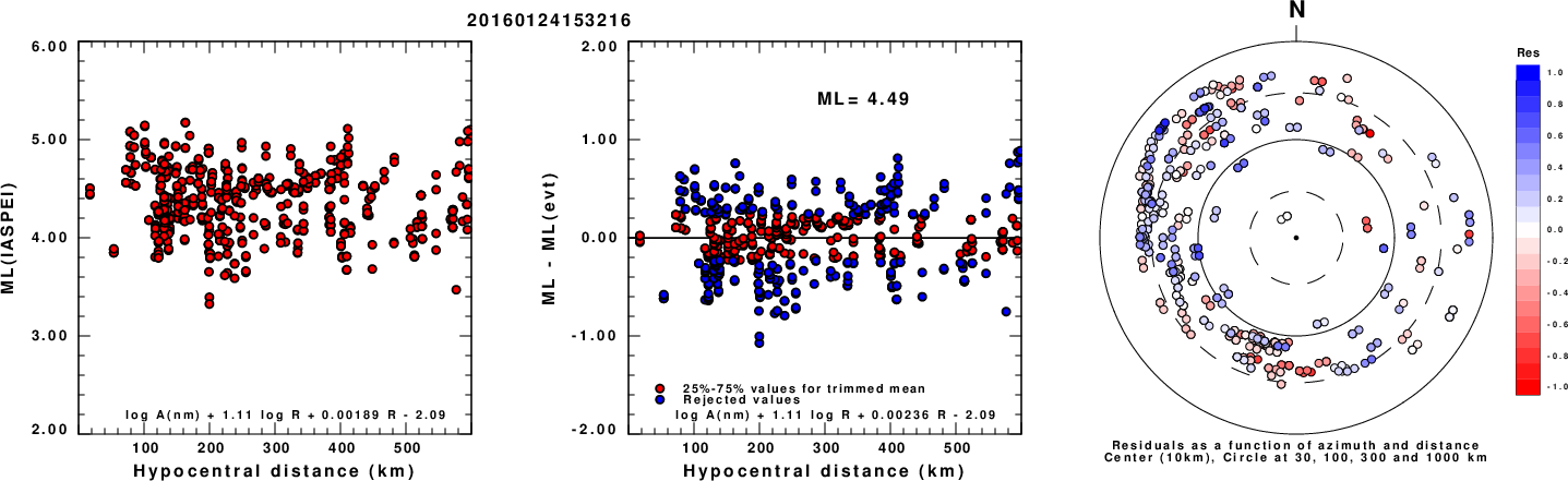
Left: ML computed using the IASPEI formula for Horizontal components. Center: ML residuals computed using a modified IASPEI formula that accounts for path specific attenuation; the values used for the trimmed mean are indicated. The ML relation used for each figure is given at the bottom of each plot.
Right: Residuals from new relation as a function of distance and azimuth.
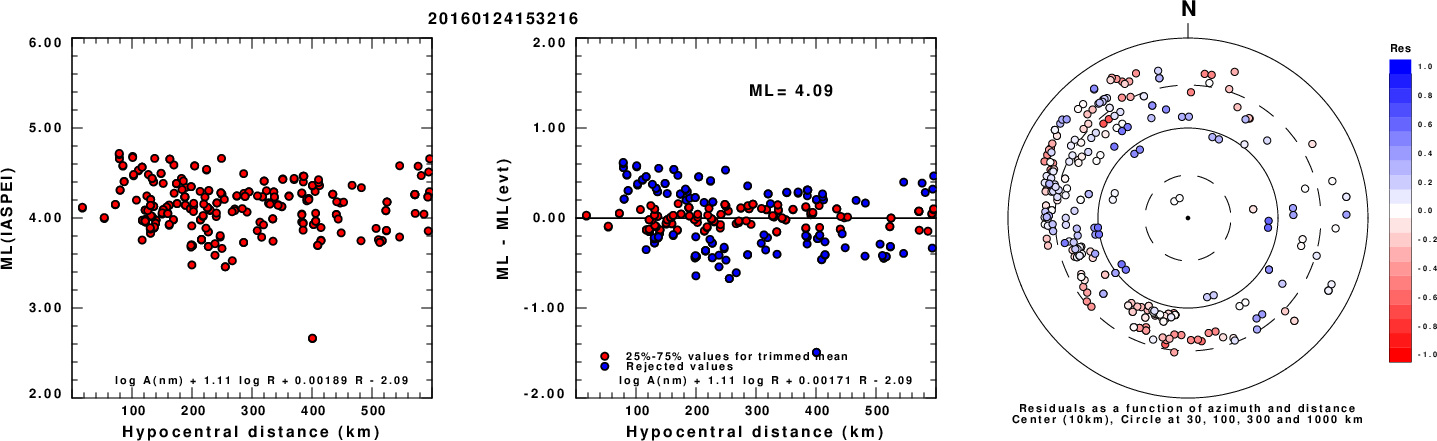
Left: ML computed using the IASPEI formula for Vertical components (research). Center: ML residuals computed using a modified IASPEI formula that accounts for path specific attenuation; the values used for the trimmed mean are indicated. The ML relation used for each figure is given at the bottom of each plot.
Right: Residuals from new relation as a function of distance and azimuth.
Context
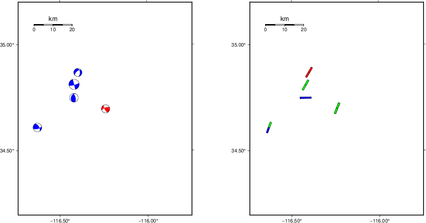
The left panel of the next figure presents the focal mechanism for this earthquake (red) in the context of other nearby events (blue) in the SLU Moment Tensor Catalog. The right panel shows the inferred direction of maximum compressive stress and the type of faulting (green is strike-slip, red is normal, blue is thrust; oblique is shown by a combination of colors). Thus context plot is useful for assessing the appropriateness of the moment tensor of this event.
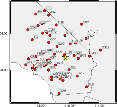
Waveform Inversion using wvfgrd96
The focal mechanism was determined using broadband seismic waveforms. The location of the event (star) and the
stations used for (red) the waveform inversion are shown in the next figure.
|
|
Location of broadband stations used for waveform inversion
|
The program wvfgrd96 was used with good traces observed at short distance to determine the focal mechanism, depth and seismic moment. This technique requires a high quality signal and well determined velocity model for the Green's functions. To the extent that these are the quality data, this type of mechanism should be preferred over the radiation pattern technique which requires the separate step of defining the pressure and tension quadrants and the correct strike.
The observed and predicted traces are filtered using the following gsac commands:
cut o DIST/3.3 -20 o DIST/3.3 +50
rtr
taper w 0.1
hp c 0.03 n 3
lp c 0.07 n 3
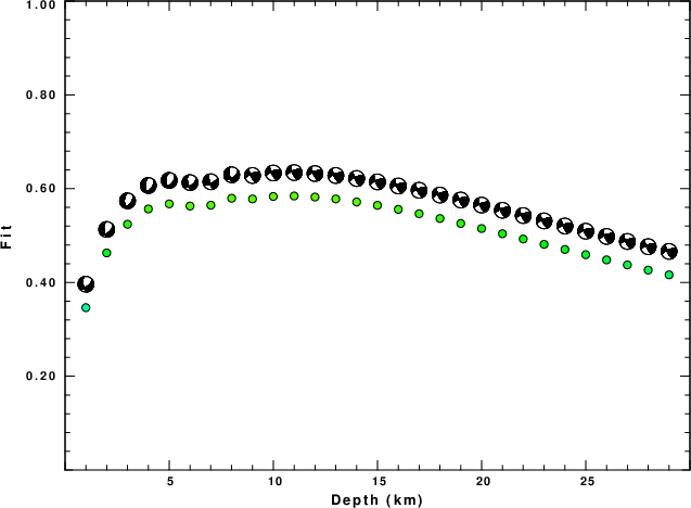
The results of this grid search are as follow:
           DEPTH  STK   DIP  RAKE   MW    FIT
WVFGRD96    1.0    55    60   -40   3.63 0.3463
WVFGRD96    2.0    50    50   -45   3.78 0.4630
WVFGRD96    3.0    40    45   -60   3.87 0.5241
WVFGRD96    4.0    40    45   -60   3.90 0.5568
WVFGRD96    5.0    40    45   -60   3.92 0.5676
WVFGRD96    6.0    55    55   -35   3.88 0.5630
WVFGRD96    7.0    65    70   -15   3.87 0.5648
WVFGRD96    8.0    55    55   -35   3.94 0.5796
WVFGRD96    9.0   250    65    20   3.93 0.5781
WVFGRD96   10.0   250    65    20   3.94 0.5834
WVFGRD96   11.0   250    65    20   3.96 0.5844
WVFGRD96   12.0   250    65    20   3.97 0.5822
WVFGRD96   13.0   250    70    20   3.98 0.5781
WVFGRD96   14.0   250    70    20   3.99 0.5717
WVFGRD96   15.0   250    70    20   4.00 0.5645
WVFGRD96   16.0   250    70    20   4.01 0.5558
WVFGRD96   17.0   250    70    20   4.02 0.5466
WVFGRD96   18.0   250    70    20   4.03 0.5364
WVFGRD96   19.0   250    70    20   4.03 0.5258
WVFGRD96   20.0   250    70    20   4.04 0.5150
WVFGRD96   21.0   250    70    20   4.05 0.5039
WVFGRD96   22.0   250    70    20   4.06 0.4927
WVFGRD96   23.0   250    70    20   4.06 0.4813
WVFGRD96   24.0   250    70    20   4.07 0.4704
WVFGRD96   25.0   250    70    20   4.08 0.4593
WVFGRD96   26.0   250    70    20   4.08 0.4482
WVFGRD96   27.0   250    70    20   4.09 0.4374
WVFGRD96   28.0   250    70    20   4.09 0.4264
WVFGRD96   29.0   250    70    20   4.10 0.4162
The best solution is
WVFGRD96 11.0 250 65 20 3.96 0.5844
The mechanism corresponding to the best fit is
|
|
Figure 1. Waveform inversion focal mechanism
|
The best fit as a function of depth is given in the following figure:
|
|
Figure 2. Depth sensitivity for waveform mechanism
|
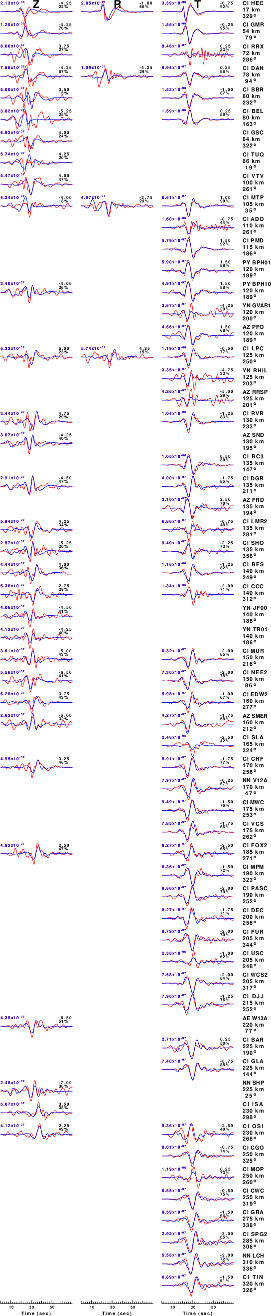
The comparison of the observed and predicted waveforms is given in the next figure. The red traces are the observed and the blue are the predicted.
Each observed-predicted component is plotted to the same scale and peak amplitudes are indicated by the numbers to the left of each trace. A pair of numbers is given in black at the right of each predicted traces. The upper number it the time shift required for maximum correlation between the observed and predicted traces. This time shift is required because the synthetics are not computed at exactly the same distance as the observed, the velocity model used in the predictions may not be perfect and the epicentral parameters may be be off.
A positive time shift indicates that the prediction is too fast and should be delayed to match the observed trace (shift to the right in this figure). A negative value indicates that the prediction is too slow. The lower number gives the percentage of variance reduction to characterize the individual goodness of fit (100% indicates a perfect fit).
The bandpass filter used in the processing and for the display was
cut o DIST/3.3 -20 o DIST/3.3 +50
rtr
taper w 0.1
hp c 0.03 n 3
lp c 0.07 n 3
|
|
Figure 3. Waveform comparison for selected depth. Red: observed; Blue - predicted. The time shift with respect to the model prediction is indicated. The percent of fit is also indicated. The time scale is relative to the first trace sample.
|
|
|
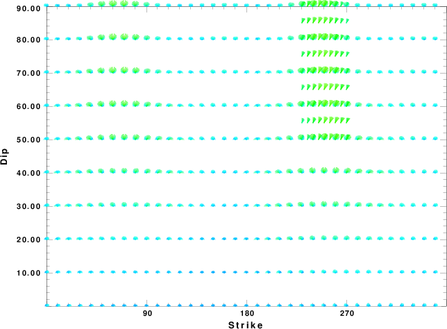
Focal mechanism sensitivity at the preferred depth. The red color indicates a very good fit to the waveforms.
Each solution is plotted as a vector at a given value of strike and dip with the angle of the vector representing the rake angle, measured, with respect to the upward vertical (N) in the figure.
|
A check on the assumed source location is possible by looking at the time shifts between the observed and predicted traces. The time shifts for waveform matching arise for several reasons:
- The origin time and epicentral distance are incorrect
- The velocity model used for the inversion is incorrect
- The velocity model used to define the P-arrival time is not the
same as the velocity model used for the waveform inversion
(assuming that the initial trace alignment is based on the
P arrival time)
Assuming only a mislocation, the time shifts are fit to a functional form:
Time_shift = A + B cos Azimuth + C Sin Azimuth
The time shifts for this inversion lead to the next figure:
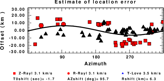
The derived shift in origin time and epicentral coordinates are given at the bottom of the figure.
Velocity Model
The WUS.model used for the waveform synthetic seismograms and for the surface wave eigenfunctions and dispersion is as follows
(The format is in the model96 format of Computer Programs in Seismology).
MODEL.01
Model after     8 iterations
ISOTROPIC
KGS
FLAT EARTH
1-D
CONSTANT VELOCITY
LINE08
LINE09
LINE10
LINE11
      H(KM)   VP(KM/S)   VS(KM/S) RHO(GM/CC)         QP         QS       ETAP       ETAS      FREFP      FREFS
     1.9000     3.4065     2.0089     2.2150  0.302E-02  0.679E-02   0.00       0.00       1.00       1.00
     6.1000     5.5445     3.2953     2.6089  0.349E-02  0.784E-02   0.00       0.00       1.00       1.00
    13.0000     6.2708     3.7396     2.7812  0.212E-02  0.476E-02   0.00       0.00       1.00       1.00
    19.0000     6.4075     3.7680     2.8223  0.111E-02  0.249E-02   0.00       0.00       1.00       1.00
     0.0000     7.9000     4.6200     3.2760  0.164E-10  0.370E-10   0.00       0.00       1.00       1.00
Last Changed Fri Apr 26 01:27:06 PM CDT 2024