Location
Location ANSS
The ANSS event ID is ak01613v15nv and the event page is at
https://earthquake.usgs.gov/earthquakes/eventpage/ak01613v15nv/executive.
2016/01/24 10:30:30 59.620 -153.339 125.6 7.1 Alaska
Focal Mechanism
 USGS/SLU Moment Tensor Solution
 ENS  2016/01/24 10:30:30:0  59.62 -153.34 125.6 7.1 Alaska

 Stations used:
   AK.CAST AK.DIV AK.KTH AK.MCK AK.PPLA AT.OHAK AT.PMR AT.TTA
   II.KDAK TA.L19K TA.N19K TA.O18K TA.O19K TA.P18K

 Filtering commands used:
   cut o DIST/3.3 -60 o DIST/3.3 +180
   rtr
   taper w 0.1
   hp c 0.01 n 3
   lp c 0.025 n 3

 Best Fitting Double Couple
  Mo = 4.42e+26 dyne-cm
  Mw = 7.03
  Z  = 114 km
  Plane   Strike  Dip  Rake
   NP1       55    65    30
   NP2      311    63   152
  Principal Axes:
   Axis    Value   Plunge  Azimuth
    T   4.42e+26     38     274
    N   0.00e+00     52      91
    P  -4.42e+26      1     183

 Moment Tensor: (dyne-cm)
    Component   Value
       Mxx    -4.39e+26
       Mxy    -3.91e+25
       Mxz     2.36e+25
       Myy     2.70e+26
       Myz    -2.14e+26
       Mzz     1.69e+26


                     --------------
                 ----------------------
              ----------------------------
             ------------------------------
           ###########-----------------------
          ###############--------------------#
         ###################----------------###
        #######################------------#####
        #########################---------######
       #######   ##################-----#########
       ####### T ####################--##########
       #######   ####################-###########
       ############################-----#########
        ########################---------#######
        ######################------------######
         ##################---------------#####
          ############---------------------###
           -##-----------------------------##
             ------------------------------
              ----------------------------
                 ---------   ----------
                     ----- P ------


 Global CMT Convention Moment Tensor:
      R          T          P
  1.69e+26   2.36e+25   2.14e+26
  2.36e+25  -4.39e+26   3.91e+25
  2.14e+26   3.91e+25   2.70e+26


Details of the solution is found at

http://www.eas.slu.edu/eqc/eqc_mt/MECH.NA/20160124103030/index.html
|
Preferred Solution
The preferred solution from an analysis of the surface-wave spectral amplitude radiation pattern, waveform inversion or first motion observations is
      STK = 55
      DIP = 65
     RAKE = 30
       MW = 7.03
       HS = 114.0
The NDK file is 20160124103030.ndk
The waveform inversion is preferred.
Moment Tensor Comparison
The following compares this source inversion to those provided by others. The purpose is to look for major differences and also to note slight differences that might be inherent to the processing procedure. For completeness the USGS/SLU solution is repeated from above.
| SLU |
USGSMT |
USGSW |
 USGS/SLU Moment Tensor Solution
 ENS  2016/01/24 10:30:30:0  59.62 -153.34 125.6 7.1 Alaska

 Stations used:
   AK.CAST AK.DIV AK.KTH AK.MCK AK.PPLA AT.OHAK AT.PMR AT.TTA
   II.KDAK TA.L19K TA.N19K TA.O18K TA.O19K TA.P18K

 Filtering commands used:
   cut o DIST/3.3 -60 o DIST/3.3 +180
   rtr
   taper w 0.1
   hp c 0.01 n 3
   lp c 0.025 n 3

 Best Fitting Double Couple
  Mo = 4.42e+26 dyne-cm
  Mw = 7.03
  Z  = 114 km
  Plane   Strike  Dip  Rake
   NP1       55    65    30
   NP2      311    63   152
  Principal Axes:
   Axis    Value   Plunge  Azimuth
    T   4.42e+26     38     274
    N   0.00e+00     52      91
    P  -4.42e+26      1     183

 Moment Tensor: (dyne-cm)
    Component   Value
       Mxx    -4.39e+26
       Mxy    -3.91e+25
       Mxz     2.36e+25
       Myy     2.70e+26
       Myz    -2.14e+26
       Mzz     1.69e+26


                     --------------
                 ----------------------
              ----------------------------
             ------------------------------
           ###########-----------------------
          ###############--------------------#
         ###################----------------###
        #######################------------#####
        #########################---------######
       #######   ##################-----#########
       ####### T ####################--##########
       #######   ####################-###########
       ############################-----#########
        ########################---------#######
        ######################------------######
         ##################---------------#####
          ############---------------------###
           -##-----------------------------##
             ------------------------------
              ----------------------------
                 ---------   ----------
                     ----- P ------


 Global CMT Convention Moment Tensor:
      R          T          P
  1.69e+26   2.36e+25   2.14e+26
  2.36e+25  -4.39e+26   3.91e+25
  2.14e+26   3.91e+25   2.70e+26


Details of the solution is found at

http://www.eas.slu.edu/eqc/eqc_mt/MECH.NA/20160124103030/index.html
|
Body-wave Moment Tensor (Mwb)
Moment	3.867e+19 N-m
Magnitude	6.99
Depth	117.0 km
Percent DC	60%
Half Duration	–
Catalog	US (us10004gqp)
Data Source	US3
Contributor	US3
Nodal Planes
Plane	Strike	Dip	Rake
NP1	302	50	153
NP2	50	70	43
Principal Axes
Axis	Value	Plunge	Azimuth
T	4.217	45	274
N	-0.837	43	70
P	-3.381	12	172

|
W-phase Moment Tensor (Mww)
Moment	6.005e+19 N-m
Magnitude	7.12
Depth	110.5 km
Percent DC	98%
Half Duration	–
Catalog	US (us10004gqp)
Data Source	US3
Contributor	US3
Nodal Planes
Plane	Strike	Dip	Rake
NP1	313	61	152
NP2	58	66	33
Principal Axes
Axis	Value	Plunge	Azimuth
T	5.979	40	277
N	0.050	50	91
P	-6.030	3	185

|
Magnitudes
Given the availability of digital waveforms for determination of the moment tensor, this section documents the added processing leading to mLg, if appropriate to the region, and ML by application of the respective IASPEI formulae. As a research study, the linear distance term of the IASPEI formula
for ML is adjusted to remove a linear distance trend in residuals to give a regionally defined ML. The defined ML uses horizontal component recordings, but the same procedure is applied to the vertical components since there may be some interest in vertical component ground motions. Residual plots versus distance may indicate interesting features of ground motion scaling in some distance ranges. A residual plot of the regionalized magnitude is given as a function of distance and azimuth, since data sets may transcend different wave propagation provinces.
ML Magnitude
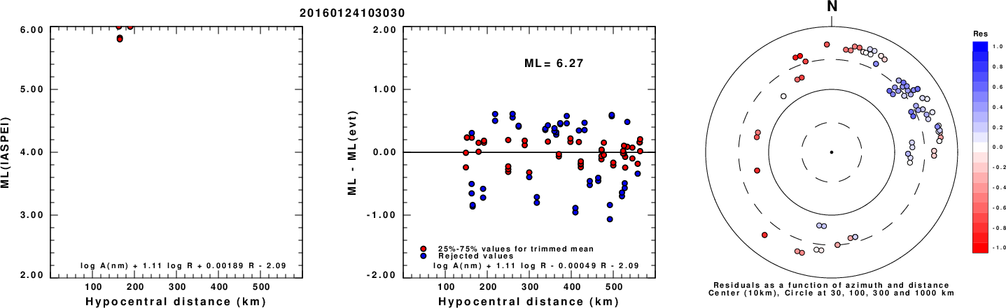
Left: ML computed using the IASPEI formula for Horizontal components. Center: ML residuals computed using a modified IASPEI formula that accounts for path specific attenuation; the values used for the trimmed mean are indicated. The ML relation used for each figure is given at the bottom of each plot.
Right: Residuals from new relation as a function of distance and azimuth.
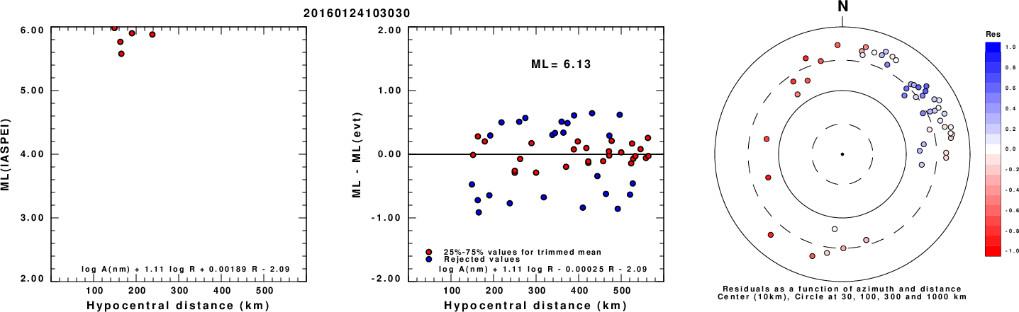
Left: ML computed using the IASPEI formula for Vertical components (research). Center: ML residuals computed using a modified IASPEI formula that accounts for path specific attenuation; the values used for the trimmed mean are indicated. The ML relation used for each figure is given at the bottom of each plot.
Right: Residuals from new relation as a function of distance and azimuth.
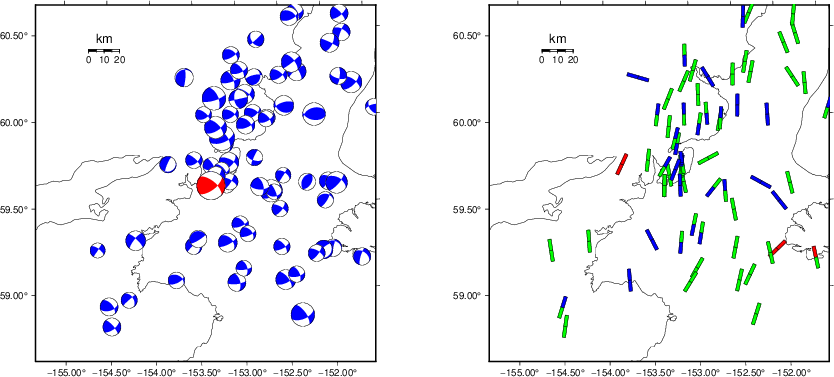
Context
The left panel of the next figure presents the focal mechanism for this earthquake (red) in the context of other nearby events (blue) in the SLU Moment Tensor Catalog. The right panel shows the inferred direction of maximum compressive stress and the type of faulting (green is strike-slip, red is normal, blue is thrust; oblique is shown by a combination of colors). Thus context plot is useful for assessing the appropriateness of the moment tensor of this event.
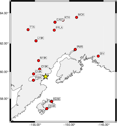
Waveform Inversion using wvfgrd96
The focal mechanism was determined using broadband seismic waveforms. The location of the event (star) and the
stations used for (red) the waveform inversion are shown in the next figure.
|
|
Location of broadband stations used for waveform inversion
|
The program wvfgrd96 was used with good traces observed at short distance to determine the focal mechanism, depth and seismic moment. This technique requires a high quality signal and well determined velocity model for the Green's functions. To the extent that these are the quality data, this type of mechanism should be preferred over the radiation pattern technique which requires the separate step of defining the pressure and tension quadrants and the correct strike.
The observed and predicted traces are filtered using the following gsac commands:
cut o DIST/3.3 -60 o DIST/3.3 +180
rtr
taper w 0.1
hp c 0.01 n 3
lp c 0.025 n 3
The results of this grid search are as follow:
           DEPTH  STK   DIP  RAKE   MW    FIT
WVFGRD96    2.0   110    40   -70   6.27 0.1895
WVFGRD96    4.0   100    40   -85   6.35 0.2190
WVFGRD96    6.0   110    45   -65   6.38 0.2218
WVFGRD96    8.0   105    45   -75   6.43 0.2338
WVFGRD96   10.0   105    40   -70   6.43 0.2129
WVFGRD96   12.0   110    40   -65   6.42 0.1842
WVFGRD96   14.0   270    85   -55   6.37 0.1723
WVFGRD96   16.0   270    85   -55   6.38 0.1829
WVFGRD96   18.0    90    90    50   6.38 0.1887
WVFGRD96   20.0   265    80   -55   6.40 0.2028
WVFGRD96   22.0   265    80   -55   6.41 0.2137
WVFGRD96   24.0   265    80   -55   6.43 0.2249
WVFGRD96   26.0   265    80   -50   6.43 0.2354
WVFGRD96   28.0   265    80   -50   6.45 0.2472
WVFGRD96   30.0   265    80   -50   6.46 0.2585
WVFGRD96   32.0   265    80   -50   6.47 0.2686
WVFGRD96   34.0   265    80   -45   6.49 0.2791
WVFGRD96   36.0   260    75   -45   6.50 0.2887
WVFGRD96   38.0   260    75   -40   6.51 0.2974
WVFGRD96   40.0   260    75   -55   6.60 0.2990
WVFGRD96   42.0   260    75   -55   6.61 0.3052
WVFGRD96   44.0   260    75   -50   6.62 0.3107
WVFGRD96   46.0   260    75   -50   6.62 0.3155
WVFGRD96   48.0   260    75   -50   6.63 0.3189
WVFGRD96   50.0   260    75   -50   6.64 0.3210
WVFGRD96   52.0   255    75   -45   6.64 0.3229
WVFGRD96   54.0   255    75   -50   6.64 0.3245
WVFGRD96   56.0   255    75   -40   6.65 0.3289
WVFGRD96   58.0   250    75   -45   6.65 0.3366
WVFGRD96   60.0    80    50    70   6.76 0.3523
WVFGRD96   62.0    75    55    65   6.77 0.3742
WVFGRD96   64.0    75    55    65   6.79 0.3999
WVFGRD96   66.0    65    55    50   6.81 0.4274
WVFGRD96   68.0    65    55    50   6.83 0.4561
WVFGRD96   70.0    65    55    50   6.84 0.4842
WVFGRD96   72.0    65    55    50   6.86 0.5110
WVFGRD96   74.0    65    55    50   6.87 0.5363
WVFGRD96   76.0    65    55    50   6.89 0.5597
WVFGRD96   78.0    60    60    40   6.89 0.5862
WVFGRD96   80.0    60    60    40   6.90 0.6121
WVFGRD96   82.0    60    60    40   6.92 0.6361
WVFGRD96   84.0    60    60    40   6.93 0.6581
WVFGRD96   86.0    60    60    40   6.94 0.6778
WVFGRD96   88.0    60    60    40   6.95 0.6948
WVFGRD96   90.0    60    60    40   6.96 0.7093
WVFGRD96   92.0    60    60    40   6.97 0.7220
WVFGRD96   94.0    60    65    40   6.97 0.7343
WVFGRD96   96.0    60    65    40   6.98 0.7455
WVFGRD96   98.0    60    65    40   6.98 0.7553
WVFGRD96  100.0    60    65    40   6.99 0.7634
WVFGRD96  102.0    60    65    35   7.00 0.7721
WVFGRD96  104.0    60    65    35   7.01 0.7792
WVFGRD96  106.0    60    65    35   7.01 0.7842
WVFGRD96  108.0    60    65    35   7.02 0.7873
WVFGRD96  110.0    60    65    35   7.02 0.7885
WVFGRD96  112.0    55    65    30   7.03 0.7908
WVFGRD96  114.0    55    65    30   7.03 0.7913
WVFGRD96  116.0    55    70    30   7.03 0.7911
WVFGRD96  118.0    55    70    30   7.03 0.7912
WVFGRD96  120.0    55    70    30   7.04 0.7898
WVFGRD96  122.0    55    70    30   7.04 0.7871
WVFGRD96  124.0    55    70    30   7.04 0.7833
WVFGRD96  126.0    55    70    30   7.04 0.7786
WVFGRD96  128.0    55    70    30   7.05 0.7730
WVFGRD96  130.0    50    70    25   7.05 0.7684
WVFGRD96  132.0    50    70    25   7.06 0.7645
WVFGRD96  134.0    50    70    25   7.06 0.7599
WVFGRD96  136.0    50    70    25   7.06 0.7546
WVFGRD96  138.0    50    75    25   7.05 0.7500
The best solution is
WVFGRD96 114.0 55 65 30 7.03 0.7913
The mechanism corresponding to the best fit is
|
|
Figure 1. Waveform inversion focal mechanism
|
The best fit as a function of depth is given in the following figure:
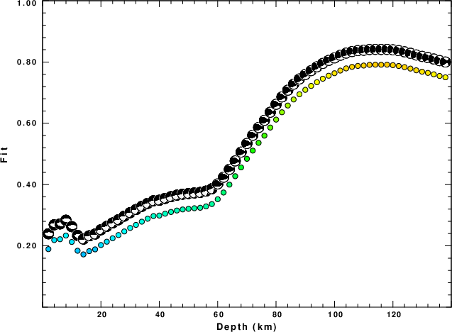
|
|
Figure 2. Depth sensitivity for waveform mechanism
|
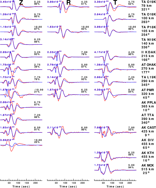
The comparison of the observed and predicted waveforms is given in the next figure. The red traces are the observed and the blue are the predicted.
Each observed-predicted component is plotted to the same scale and peak amplitudes are indicated by the numbers to the left of each trace. A pair of numbers is given in black at the right of each predicted traces. The upper number it the time shift required for maximum correlation between the observed and predicted traces. This time shift is required because the synthetics are not computed at exactly the same distance as the observed, the velocity model used in the predictions may not be perfect and the epicentral parameters may be be off.
A positive time shift indicates that the prediction is too fast and should be delayed to match the observed trace (shift to the right in this figure). A negative value indicates that the prediction is too slow. The lower number gives the percentage of variance reduction to characterize the individual goodness of fit (100% indicates a perfect fit).
The bandpass filter used in the processing and for the display was
cut o DIST/3.3 -60 o DIST/3.3 +180
rtr
taper w 0.1
hp c 0.01 n 3
lp c 0.025 n 3
|
|
Figure 3. Waveform comparison for selected depth. Red: observed; Blue - predicted. The time shift with respect to the model prediction is indicated. The percent of fit is also indicated. The time scale is relative to the first trace sample.
|
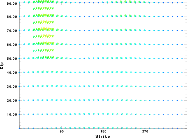
|
|
Focal mechanism sensitivity at the preferred depth. The red color indicates a very good fit to the waveforms.
Each solution is plotted as a vector at a given value of strike and dip with the angle of the vector representing the rake angle, measured, with respect to the upward vertical (N) in the figure.
|
A check on the assumed source location is possible by looking at the time shifts between the observed and predicted traces. The time shifts for waveform matching arise for several reasons:
- The origin time and epicentral distance are incorrect
- The velocity model used for the inversion is incorrect
- The velocity model used to define the P-arrival time is not the
same as the velocity model used for the waveform inversion
(assuming that the initial trace alignment is based on the
P arrival time)
Assuming only a mislocation, the time shifts are fit to a functional form:
Time_shift = A + B cos Azimuth + C Sin Azimuth
The time shifts for this inversion lead to the next figure:
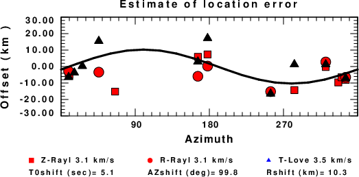
The derived shift in origin time and epicentral coordinates are given at the bottom of the figure.
Velocity Model
The WUS.model used for the waveform synthetic seismograms and for the surface wave eigenfunctions and dispersion is as follows
(The format is in the model96 format of Computer Programs in Seismology).
MODEL.01
Model after     8 iterations
ISOTROPIC
KGS
FLAT EARTH
1-D
CONSTANT VELOCITY
LINE08
LINE09
LINE10
LINE11
      H(KM)   VP(KM/S)   VS(KM/S) RHO(GM/CC)         QP         QS       ETAP       ETAS      FREFP      FREFS
     1.9000     3.4065     2.0089     2.2150  0.302E-02  0.679E-02   0.00       0.00       1.00       1.00
     6.1000     5.5445     3.2953     2.6089  0.349E-02  0.784E-02   0.00       0.00       1.00       1.00
    13.0000     6.2708     3.7396     2.7812  0.212E-02  0.476E-02   0.00       0.00       1.00       1.00
    19.0000     6.4075     3.7680     2.8223  0.111E-02  0.249E-02   0.00       0.00       1.00       1.00
     0.0000     7.9000     4.6200     3.2760  0.164E-10  0.370E-10   0.00       0.00       1.00       1.00
Last Changed Fri Apr 26 01:22:26 PM CDT 2024