Location
Location ANSS
The ANSS event ID is uw61114971 and the event page is at
https://earthquake.usgs.gov/earthquakes/eventpage/uw61114971/executive.
2015/12/30 07:39:29 48.587 -123.300 52.4 4.79 BC, Canada
Focal Mechanism
 USGS/SLU Moment Tensor Solution
 ENS  2015/12/30 07:39:29:0  48.59 -123.30  52.4 4.8 BC, Canada

 Stations used:
   CC.CIHL CC.CPCO CC.JRO CC.NORM CC.SHRK CC.SWNB CN.LLLB
   CN.PNT CN.WALA IU.COR IW.PLID MB.JTMT TA.A04D TA.B05D
   TA.C06D TA.D03D TA.E04D TA.F04D TA.F05D TA.G03D TA.G05D
   TA.I02E TA.I03D TA.I05D TA.J05D TA.K02D TD.TD009 TD.TD012
   TD.TD028 UO.BUCK UO.DBO UO.PINE US.BMO US.HAWA US.NEW
   US.NLWA UW.BABR UW.BLOW UW.BRAN UW.CCRK UW.DAVN UW.DDRF
   UW.DOSE UW.FORK UW.GNW UW.HEBO UW.HOOD UW.KENT UW.LEBA
   UW.LTY UW.OMAK UW.PASS UW.PHIN UW.RATT UW.SP2 UW.STOR
   UW.TOLT UW.TREE UW.TUCA UW.UMAT UW.WISH UW.WOLL

 Filtering commands used:
   cut o DIST/3.3 -30 o DIST/3.3 +80
   rtr
   taper w 0.1
   hp c 0.02 n 3
   lp c 0.06 n 3

 Best Fitting Double Couple
  Mo = 1.23e+23 dyne-cm
  Mw = 4.66
  Z  = 52 km
  Plane   Strike  Dip  Rake
   NP1      325    60   -109
   NP2      180    35   -60
  Principal Axes:
   Axis    Value   Plunge  Azimuth
    T   1.23e+23     13      69
    N   0.00e+00     17     335
    P  -1.23e+23     69     195

 Moment Tensor: (dyne-cm)
    Component   Value
       Mxx    -6.17e+15
       Mxy     3.53e+22
       Mxz     5.04e+22
       Myy     1.00e+23
       Myz     3.64e+22
       Mzz    -1.00e+23


                     ----##########
                 -----#################
              ######-#####################
             ######-----###################
           #######---------##################
          #######------------#################
         #######---------------############   #
        #######------------------########## T ##
        #######-------------------#########   ##
       ########--------------------##############
       #######----------------------#############
       #######-----------------------############
       ########----------   ----------###########
        #######---------- P -----------#########
        #######----------   -----------#########
         #######------------------------#######
          #######-----------------------######
           #######----------------------#####
             ######---------------------###
              ######--------------------##
                 #####-----------------
                     ####----------


 Global CMT Convention Moment Tensor:
      R          T          P
 -1.00e+23   5.04e+22  -3.64e+22
  5.04e+22  -6.17e+15  -3.53e+22
 -3.64e+22  -3.53e+22   1.00e+23


Details of the solution is found at

http://www.eas.slu.edu/eqc/eqc_mt/MECH.NA/20151230073929/index.html
|
Preferred Solution
The preferred solution from an analysis of the surface-wave spectral amplitude radiation pattern, waveform inversion or first motion observations is
      STK = 180
      DIP = 35
     RAKE = -60
       MW = 4.66
       HS = 52.0
The NDK file is 20151230073929.ndk
The waveform inversion is preferred.
Moment Tensor Comparison
The following compares this source inversion to those provided by others. The purpose is to look for major differences and also to note slight differences that might be inherent to the processing procedure. For completeness the USGS/SLU solution is repeated from above.
| SLU |
USGSMT |
USGSW |
 USGS/SLU Moment Tensor Solution
 ENS  2015/12/30 07:39:29:0  48.59 -123.30  52.4 4.8 BC, Canada

 Stations used:
   CC.CIHL CC.CPCO CC.JRO CC.NORM CC.SHRK CC.SWNB CN.LLLB
   CN.PNT CN.WALA IU.COR IW.PLID MB.JTMT TA.A04D TA.B05D
   TA.C06D TA.D03D TA.E04D TA.F04D TA.F05D TA.G03D TA.G05D
   TA.I02E TA.I03D TA.I05D TA.J05D TA.K02D TD.TD009 TD.TD012
   TD.TD028 UO.BUCK UO.DBO UO.PINE US.BMO US.HAWA US.NEW
   US.NLWA UW.BABR UW.BLOW UW.BRAN UW.CCRK UW.DAVN UW.DDRF
   UW.DOSE UW.FORK UW.GNW UW.HEBO UW.HOOD UW.KENT UW.LEBA
   UW.LTY UW.OMAK UW.PASS UW.PHIN UW.RATT UW.SP2 UW.STOR
   UW.TOLT UW.TREE UW.TUCA UW.UMAT UW.WISH UW.WOLL

 Filtering commands used:
   cut o DIST/3.3 -30 o DIST/3.3 +80
   rtr
   taper w 0.1
   hp c 0.02 n 3
   lp c 0.06 n 3

 Best Fitting Double Couple
  Mo = 1.23e+23 dyne-cm
  Mw = 4.66
  Z  = 52 km
  Plane   Strike  Dip  Rake
   NP1      325    60   -109
   NP2      180    35   -60
  Principal Axes:
   Axis    Value   Plunge  Azimuth
    T   1.23e+23     13      69
    N   0.00e+00     17     335
    P  -1.23e+23     69     195

 Moment Tensor: (dyne-cm)
    Component   Value
       Mxx    -6.17e+15
       Mxy     3.53e+22
       Mxz     5.04e+22
       Myy     1.00e+23
       Myz     3.64e+22
       Mzz    -1.00e+23


                     ----##########
                 -----#################
              ######-#####################
             ######-----###################
           #######---------##################
          #######------------#################
         #######---------------############   #
        #######------------------########## T ##
        #######-------------------#########   ##
       ########--------------------##############
       #######----------------------#############
       #######-----------------------############
       ########----------   ----------###########
        #######---------- P -----------#########
        #######----------   -----------#########
         #######------------------------#######
          #######-----------------------######
           #######----------------------#####
             ######---------------------###
              ######--------------------##
                 #####-----------------
                     ####----------


 Global CMT Convention Moment Tensor:
      R          T          P
 -1.00e+23   5.04e+22  -3.64e+22
  5.04e+22  -6.17e+15  -3.53e+22
 -3.64e+22  -3.53e+22   1.00e+23


Details of the solution is found at

http://www.eas.slu.edu/eqc/eqc_mt/MECH.NA/20151230073929/index.html
|
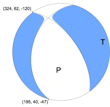
Regional Moment Tensor (Mwr)
Moment	1.278e+16 N-m
Magnitude	4.67
Depth	52.0 km
Percent DC	98%
Half Duration	–
Catalog	US (us10004adm)
Data Source	US3
Contributor	US3
Nodal Planes
Plane	Strike	Dip	Rake
NP1	195	40	-47
NP2	324	62	-120
Principal Axes
Axis	Value	Plunge	Azimuth
T	1.285	12	75
N	-0.015	26	339
P	-1.271	61	189
|
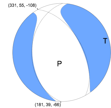
W-phase Moment Tensor (Mww)
Moment	1.495e+16 N-m
Magnitude	4.72
Depth	45.5 km
Percent DC	83%
Half Duration	–
Catalog	US (us10004adm)
Data Source	US3
Contributor	US3
Nodal Planes
Plane	Strike	Dip	Rake
NP1	181	39	-66
NP2	331	55	-108
Principal Axes
Axis	Value	Plunge	Azimuth
T	1.558	8	74
N	-0.135	15	342
P	-1.423	73	193
|
Magnitudes
Given the availability of digital waveforms for determination of the moment tensor, this section documents the added processing leading to mLg, if appropriate to the region, and ML by application of the respective IASPEI formulae. As a research study, the linear distance term of the IASPEI formula
for ML is adjusted to remove a linear distance trend in residuals to give a regionally defined ML. The defined ML uses horizontal component recordings, but the same procedure is applied to the vertical components since there may be some interest in vertical component ground motions. Residual plots versus distance may indicate interesting features of ground motion scaling in some distance ranges. A residual plot of the regionalized magnitude is given as a function of distance and azimuth, since data sets may transcend different wave propagation provinces.
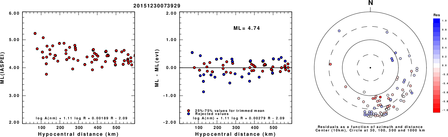
ML Magnitude
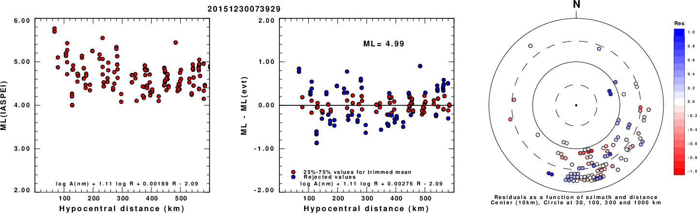
Left: ML computed using the IASPEI formula for Horizontal components. Center: ML residuals computed using a modified IASPEI formula that accounts for path specific attenuation; the values used for the trimmed mean are indicated. The ML relation used for each figure is given at the bottom of each plot.
Right: Residuals from new relation as a function of distance and azimuth.
Left: ML computed using the IASPEI formula for Vertical components (research). Center: ML residuals computed using a modified IASPEI formula that accounts for path specific attenuation; the values used for the trimmed mean are indicated. The ML relation used for each figure is given at the bottom of each plot.
Right: Residuals from new relation as a function of distance and azimuth.
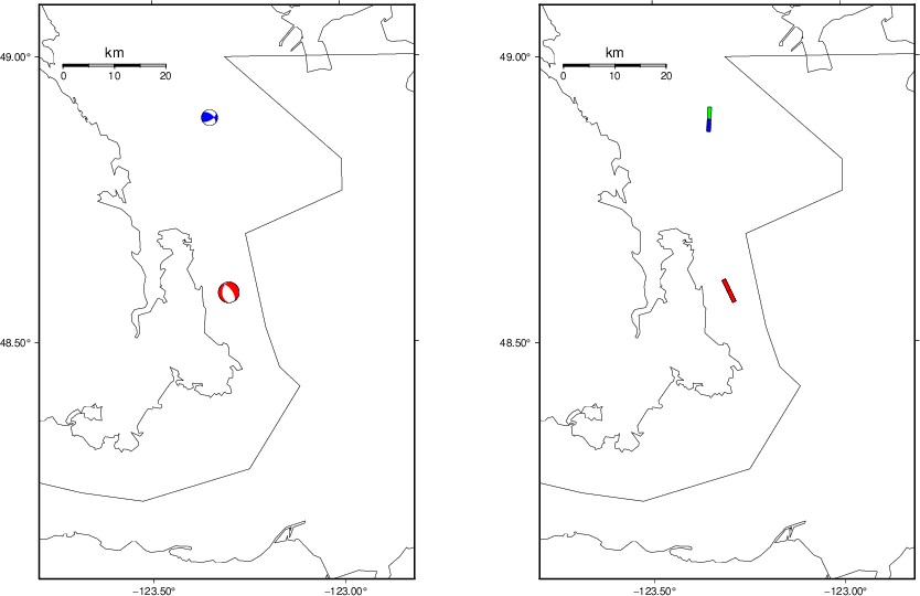
Context
The left panel of the next figure presents the focal mechanism for this earthquake (red) in the context of other nearby events (blue) in the SLU Moment Tensor Catalog. The right panel shows the inferred direction of maximum compressive stress and the type of faulting (green is strike-slip, red is normal, blue is thrust; oblique is shown by a combination of colors). Thus context plot is useful for assessing the appropriateness of the moment tensor of this event.
Waveform Inversion using wvfgrd96
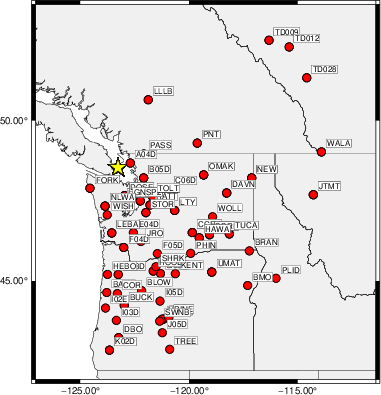
The focal mechanism was determined using broadband seismic waveforms. The location of the event (star) and the
stations used for (red) the waveform inversion are shown in the next figure.
|
|
Location of broadband stations used for waveform inversion
|
The program wvfgrd96 was used with good traces observed at short distance to determine the focal mechanism, depth and seismic moment. This technique requires a high quality signal and well determined velocity model for the Green's functions. To the extent that these are the quality data, this type of mechanism should be preferred over the radiation pattern technique which requires the separate step of defining the pressure and tension quadrants and the correct strike.
The observed and predicted traces are filtered using the following gsac commands:
cut o DIST/3.3 -30 o DIST/3.3 +80
rtr
taper w 0.1
hp c 0.02 n 3
lp c 0.06 n 3
The results of this grid search are as follow:
           DEPTH  STK   DIP  RAKE   MW    FIT
WVFGRD96    2.0   160    40    90   4.04 0.3498
WVFGRD96    4.0   160    50   -85   4.11 0.3102
WVFGRD96    6.0   190    60   -50   4.07 0.2675
WVFGRD96    8.0   150    80    70   4.15 0.2920
WVFGRD96   10.0   150    80    70   4.17 0.3280
WVFGRD96   12.0   215    25   -15   4.18 0.3671
WVFGRD96   14.0   210    30   -25   4.20 0.4003
WVFGRD96   16.0   210    30   -25   4.22 0.4311
WVFGRD96   18.0   210    30   -25   4.24 0.4567
WVFGRD96   20.0   210    30   -25   4.26 0.4787
WVFGRD96   22.0   210    30   -20   4.29 0.4980
WVFGRD96   24.0   210    30   -20   4.31 0.5155
WVFGRD96   26.0   210    30   -20   4.33 0.5317
WVFGRD96   28.0   210    30   -20   4.35 0.5482
WVFGRD96   30.0   210    35   -20   4.37 0.5633
WVFGRD96   32.0   210    35   -20   4.39 0.5767
WVFGRD96   34.0   205    35   -30   4.40 0.5897
WVFGRD96   36.0   195    35   -40   4.41 0.6035
WVFGRD96   38.0   190    30   -50   4.42 0.6174
WVFGRD96   40.0   185    30   -55   4.56 0.6543
WVFGRD96   42.0   180    30   -60   4.58 0.6708
WVFGRD96   44.0   180    30   -60   4.60 0.6822
WVFGRD96   46.0   180    35   -60   4.61 0.6909
WVFGRD96   48.0   180    35   -60   4.63 0.6998
WVFGRD96   50.0   180    35   -60   4.65 0.7052
WVFGRD96   52.0   180    35   -60   4.66 0.7079
WVFGRD96   54.0   180    35   -60   4.67 0.7076
WVFGRD96   56.0   185    40   -55   4.69 0.7046
WVFGRD96   58.0   185    40   -55   4.70 0.7026
WVFGRD96   60.0   185    40   -55   4.71 0.6985
WVFGRD96   62.0   185    40   -55   4.72 0.6913
WVFGRD96   64.0   185    40   -55   4.73 0.6819
WVFGRD96   66.0   185    40   -55   4.74 0.6702
WVFGRD96   68.0   190    45   -50   4.75 0.6596
WVFGRD96   70.0   190    45   -50   4.76 0.6489
WVFGRD96   72.0   190    45   -50   4.76 0.6365
WVFGRD96   74.0   190    45   -50   4.77 0.6228
WVFGRD96   76.0   190    45   -50   4.77 0.6085
WVFGRD96   78.0   190    45   -45   4.78 0.5939
WVFGRD96   80.0   190    50   -45   4.79 0.5804
WVFGRD96   82.0   190    50   -45   4.79 0.5688
WVFGRD96   84.0   190    50   -45   4.80 0.5560
WVFGRD96   86.0   190    50   -45   4.80 0.5422
WVFGRD96   88.0   190    50   -45   4.80 0.5282
WVFGRD96   90.0   195    50   -40   4.80 0.5147
WVFGRD96   92.0   195    50   -40   4.80 0.5014
WVFGRD96   94.0   195    55   -40   4.81 0.4879
WVFGRD96   96.0   195    55   -40   4.81 0.4766
WVFGRD96   98.0   200    55   -30   4.81 0.4655
The best solution is
WVFGRD96 52.0 180 35 -60 4.66 0.7079
The mechanism corresponding to the best fit is
|
|
Figure 1. Waveform inversion focal mechanism
|
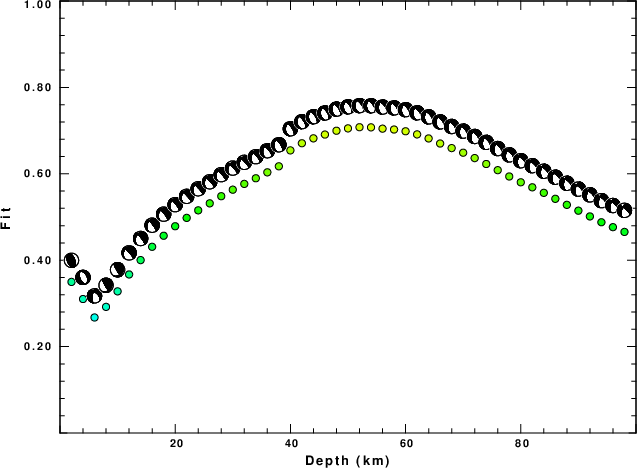
The best fit as a function of depth is given in the following figure:
|
|
Figure 2. Depth sensitivity for waveform mechanism
|
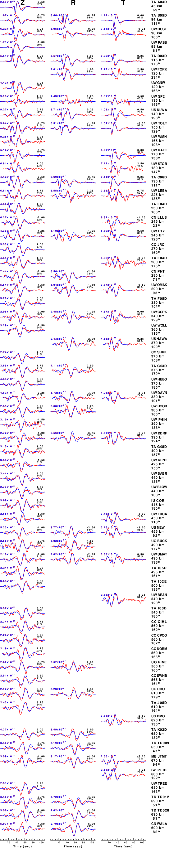
The comparison of the observed and predicted waveforms is given in the next figure. The red traces are the observed and the blue are the predicted.
Each observed-predicted component is plotted to the same scale and peak amplitudes are indicated by the numbers to the left of each trace. A pair of numbers is given in black at the right of each predicted traces. The upper number it the time shift required for maximum correlation between the observed and predicted traces. This time shift is required because the synthetics are not computed at exactly the same distance as the observed, the velocity model used in the predictions may not be perfect and the epicentral parameters may be be off.
A positive time shift indicates that the prediction is too fast and should be delayed to match the observed trace (shift to the right in this figure). A negative value indicates that the prediction is too slow. The lower number gives the percentage of variance reduction to characterize the individual goodness of fit (100% indicates a perfect fit).
The bandpass filter used in the processing and for the display was
cut o DIST/3.3 -30 o DIST/3.3 +80
rtr
taper w 0.1
hp c 0.02 n 3
lp c 0.06 n 3
|
|
Figure 3. Waveform comparison for selected depth. Red: observed; Blue - predicted. The time shift with respect to the model prediction is indicated. The percent of fit is also indicated. The time scale is relative to the first trace sample.
|
|
|
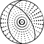
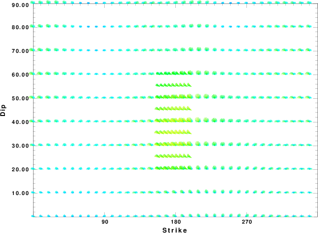
Focal mechanism sensitivity at the preferred depth. The red color indicates a very good fit to the waveforms.
Each solution is plotted as a vector at a given value of strike and dip with the angle of the vector representing the rake angle, measured, with respect to the upward vertical (N) in the figure.
|
A check on the assumed source location is possible by looking at the time shifts between the observed and predicted traces. The time shifts for waveform matching arise for several reasons:
- The origin time and epicentral distance are incorrect
- The velocity model used for the inversion is incorrect
- The velocity model used to define the P-arrival time is not the
same as the velocity model used for the waveform inversion
(assuming that the initial trace alignment is based on the
P arrival time)
Assuming only a mislocation, the time shifts are fit to a functional form:
Time_shift = A + B cos Azimuth + C Sin Azimuth
The time shifts for this inversion lead to the next figure:
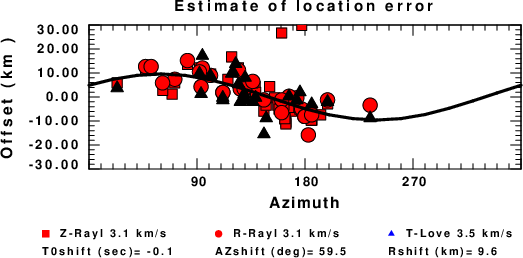
The derived shift in origin time and epicentral coordinates are given at the bottom of the figure.
Velocity Model
The WUS.model used for the waveform synthetic seismograms and for the surface wave eigenfunctions and dispersion is as follows
(The format is in the model96 format of Computer Programs in Seismology).
MODEL.01
Model after     8 iterations
ISOTROPIC
KGS
FLAT EARTH
1-D
CONSTANT VELOCITY
LINE08
LINE09
LINE10
LINE11
      H(KM)   VP(KM/S)   VS(KM/S) RHO(GM/CC)         QP         QS       ETAP       ETAS      FREFP      FREFS
     1.9000     3.4065     2.0089     2.2150  0.302E-02  0.679E-02   0.00       0.00       1.00       1.00
     6.1000     5.5445     3.2953     2.6089  0.349E-02  0.784E-02   0.00       0.00       1.00       1.00
    13.0000     6.2708     3.7396     2.7812  0.212E-02  0.476E-02   0.00       0.00       1.00       1.00
    19.0000     6.4075     3.7680     2.8223  0.111E-02  0.249E-02   0.00       0.00       1.00       1.00
     0.0000     7.9000     4.6200     3.2760  0.164E-10  0.370E-10   0.00       0.00       1.00       1.00
Last Changed Sat Apr 27 02:24:44 AM CDT 2024