Location
Location ANSS
The ANSS event ID is ak01581sc69w and the event page is at
https://earthquake.usgs.gov/earthquakes/eventpage/ak01581sc69w/executive.
2015/06/24 22:32:20 61.664 -151.962 114.2 5.8 Alaska
Focal Mechanism
 USGS/SLU Moment Tensor Solution
 ENS  2015/06/24 22:32:20:0  61.66 -151.96 114.2 5.8 Alaska

 Stations used:
   AK.BPAW AK.BRLK AK.BWN AK.CAPN AK.CCB AK.CNP AK.CUT AK.FID
   AK.FIRE AK.GLB AK.GLI AK.HDA AK.HIN AK.KLU AK.KNK AK.KTH
   AK.MCAR AK.MCK AK.MDM AK.MLY AK.NEA2 AK.PPD AK.PWL AK.RC01
   AK.RND AK.SAW AK.SCM AK.SCRK AK.SKN AK.SSN AK.TRF AK.VRDI
   AK.WRH II.KDAK IU.COLA TA.I23K TA.K27K TA.L27K TA.M24K
   TA.N25K TA.O22K TA.POKR

 Filtering commands used:
   cut o DIST/3.3 -30 o DIST/3.3 +70
   rtr
   taper w 0.1
   hp c 0.02 n 3
   lp c 0.06 n 3

 Best Fitting Double Couple
  Mo = 6.76e+24 dyne-cm
  Mw = 5.82
  Z  = 122 km
  Plane   Strike  Dip  Rake
   NP1      296    54   110
   NP2       85    40    65
  Principal Axes:
   Axis    Value   Plunge  Azimuth
    T   6.76e+24     72     258
    N   0.00e+00     16     105
    P  -6.76e+24      7      13

 Moment Tensor: (dyne-cm)
    Component   Value
       Mxx    -6.31e+24
       Mxy    -1.28e+24
       Mxz    -1.25e+24
       Myy     2.73e+23
       Myz    -2.09e+24
       Mzz     6.03e+24


                     ---------- P -
                 --------------   -----
              ----------------------------
             ------------------------------
           ----------------------------------
          -################-------------------
         ######################----------------
        ###########################-------------
        ##############################----------
       #################################---------
       ###############   #################------#
       ############### T ##################-----#
       -##############   ###################--###
        -#######################################
        ---################################---##
         ----############################-----#
          ------#####################---------
           -----------##########-------------
             ------------------------------
              ----------------------------
                 ----------------------
                     --------------


 Global CMT Convention Moment Tensor:
      R          T          P
  6.03e+24  -1.25e+24   2.09e+24
 -1.25e+24  -6.31e+24   1.28e+24
  2.09e+24   1.28e+24   2.73e+23


Details of the solution is found at

http://www.eas.slu.edu/eqc/eqc_mt/MECH.NA/20150624223220/index.html
|
Preferred Solution
The preferred solution from an analysis of the surface-wave spectral amplitude radiation pattern, waveform inversion or first motion observations is
      STK = 85
      DIP = 40
     RAKE = 65
       MW = 5.82
       HS = 122.0
The NDK file is 20150624223220.ndk
The waveform inversion is preferred.
Moment Tensor Comparison
The following compares this source inversion to those provided by others. The purpose is to look for major differences and also to note slight differences that might be inherent to the processing procedure. For completeness the USGS/SLU solution is repeated from above.
| SLU |
USGSMT |
GCMT |
USGSW |
USGSCMT |
 USGS/SLU Moment Tensor Solution
 ENS  2015/06/24 22:32:20:0  61.66 -151.96 114.2 5.8 Alaska

 Stations used:
   AK.BPAW AK.BRLK AK.BWN AK.CAPN AK.CCB AK.CNP AK.CUT AK.FID
   AK.FIRE AK.GLB AK.GLI AK.HDA AK.HIN AK.KLU AK.KNK AK.KTH
   AK.MCAR AK.MCK AK.MDM AK.MLY AK.NEA2 AK.PPD AK.PWL AK.RC01
   AK.RND AK.SAW AK.SCM AK.SCRK AK.SKN AK.SSN AK.TRF AK.VRDI
   AK.WRH II.KDAK IU.COLA TA.I23K TA.K27K TA.L27K TA.M24K
   TA.N25K TA.O22K TA.POKR

 Filtering commands used:
   cut o DIST/3.3 -30 o DIST/3.3 +70
   rtr
   taper w 0.1
   hp c 0.02 n 3
   lp c 0.06 n 3

 Best Fitting Double Couple
  Mo = 6.76e+24 dyne-cm
  Mw = 5.82
  Z  = 122 km
  Plane   Strike  Dip  Rake
   NP1      296    54   110
   NP2       85    40    65
  Principal Axes:
   Axis    Value   Plunge  Azimuth
    T   6.76e+24     72     258
    N   0.00e+00     16     105
    P  -6.76e+24      7      13

 Moment Tensor: (dyne-cm)
    Component   Value
       Mxx    -6.31e+24
       Mxy    -1.28e+24
       Mxz    -1.25e+24
       Myy     2.73e+23
       Myz    -2.09e+24
       Mzz     6.03e+24


                     ---------- P -
                 --------------   -----
              ----------------------------
             ------------------------------
           ----------------------------------
          -################-------------------
         ######################----------------
        ###########################-------------
        ##############################----------
       #################################---------
       ###############   #################------#
       ############### T ##################-----#
       -##############   ###################--###
        -#######################################
        ---################################---##
         ----############################-----#
          ------#####################---------
           -----------##########-------------
             ------------------------------
              ----------------------------
                 ----------------------
                     --------------


 Global CMT Convention Moment Tensor:
      R          T          P
  6.03e+24  -1.25e+24   2.09e+24
 -1.25e+24  -6.31e+24   1.28e+24
  2.09e+24   1.28e+24   2.73e+23


Details of the solution is found at

http://www.eas.slu.edu/eqc/eqc_mt/MECH.NA/20150624223220/index.html
|
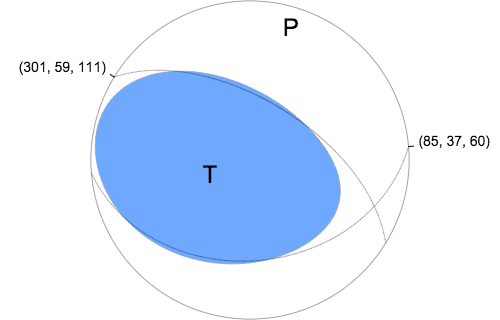
Regional Moment Tensor (Mwr)
Moment	6.017e+17 N-m
Magnitude	5.79
Depth	114.0 km
Percent DC	71%
Half Duration	-
Catalog	US (us10002lgv)
Data Source	US3
Contributor	US3
Nodal Planes
Plane	Strike	Dip	Rake
NP1	301	59	111
NP2	85	37	60
Principal Axes
Axis	Value	Plunge	Azimuth
T	6.428	69	255
N	-0.930	18	110
P	-5.498	12	17
|
une 24, 2015, SOUTHERN ALASKA, MW=5.8

Howard Koss

CENTROID-MOMENT-TENSOR  SOLUTION
GCMT EVENT:     C201506242232A
DATA: II IU DK CU MN G  IC LD GE
 XF KP
L.P.BODY WAVES:157S, 336C, T= 40
MANTLE WAVES:   65S,  76C, T=125
SURFACE WAVES: 168S, 391C, T= 50
TIMESTAMP:      Q-20150625080531
CENTROID LOCATION:
ORIGIN TIME:      22:32:22.9 0.1
LAT:61.83N 0.01;LON:152.01W 0.01
DEP:125.5  0.5;TRIANG HDUR:  2.0
MOMENT TENSOR: SCALE 10**24 D-CM
RR= 5.500 0.052; TT=-6.110 0.062
PP= 0.603 0.065; RT=-1.270 0.050
RP= 3.170 0.046; TP= 1.730 0.057
PRINCIPAL AXES:
1.(T) VAL=  7.068;PLG=64;AZM=266
2.(N)      -0.201;    24;    111
3.(P)      -6.874;    10;     17
BEST DBLE.COUPLE:M0= 6.97*10**24
NP1: STRIKE= 81;DIP=41;SLIP=  52
NP2: STRIKE=307;DIP=59;SLIP= 118

            --------
        ------------ P ----
      --------------   ------
    -####----------------------
   #############----------------
  #################--------------
  ####################-----------
 #######################----------
 ##########   ############-------#
 ########## T #############-----##
 ##########   ##############---###
  -##########################-###
  ---######################---###
   -----################-------#
    ---------------------------
      -----------------------
        -------------------
            -----------
|
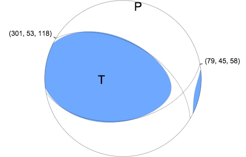
W-phase Moment Tensor (Mww)
Moment	5.642e+17 N-m
Magnitude	5.77
Depth	120.5 km
Percent DC	86%
Half Duration	-
Catalog	AK (ak11632992)
Data Source	US3
Contributor	US3
Nodal Planes
Plane	Strike	Dip	Rake
NP1	301	53	118
NP2	79	45	58
Principal Axes
Axis	Value	Plunge	Azimuth
T	5.836	67	272
N	-0.409	22	103
P	-5.426	4	11
|
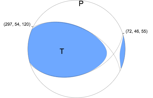
Centroid Moment Tensor (Mwc)
Moment	6.820e+17 N-m
Magnitude	5.82
Depth	105.8 km
Percent DC	89%
Half Duration	-
Catalog	US (us10002lgv)
Data Source	US3
Contributor	US3
Nodal Planes
Plane	Strike	Dip	Rake
NP1	297	54	120
NP2	72	46	55
Principal Axes
Axis	Value	Plunge	Azimuth
T	6.998	65	265
N	-0.371	24	98
P	-6.627	5	6
|
Magnitudes
Given the availability of digital waveforms for determination of the moment tensor, this section documents the added processing leading to mLg, if appropriate to the region, and ML by application of the respective IASPEI formulae. As a research study, the linear distance term of the IASPEI formula
for ML is adjusted to remove a linear distance trend in residuals to give a regionally defined ML. The defined ML uses horizontal component recordings, but the same procedure is applied to the vertical components since there may be some interest in vertical component ground motions. Residual plots versus distance may indicate interesting features of ground motion scaling in some distance ranges. A residual plot of the regionalized magnitude is given as a function of distance and azimuth, since data sets may transcend different wave propagation provinces.
ML Magnitude
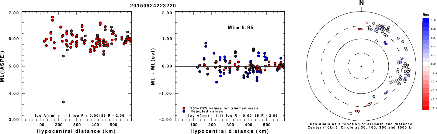
Left: ML computed using the IASPEI formula for Horizontal components. Center: ML residuals computed using a modified IASPEI formula that accounts for path specific attenuation; the values used for the trimmed mean are indicated. The ML relation used for each figure is given at the bottom of each plot.
Right: Residuals from new relation as a function of distance and azimuth.
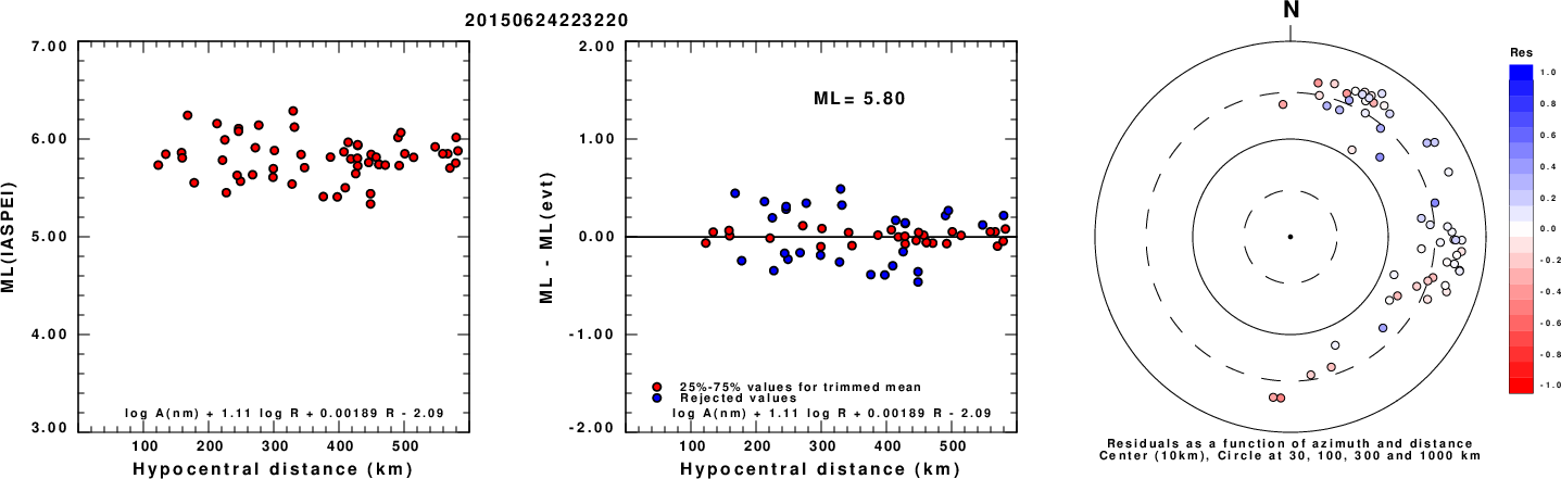
Left: ML computed using the IASPEI formula for Vertical components (research). Center: ML residuals computed using a modified IASPEI formula that accounts for path specific attenuation; the values used for the trimmed mean are indicated. The ML relation used for each figure is given at the bottom of each plot.
Right: Residuals from new relation as a function of distance and azimuth.
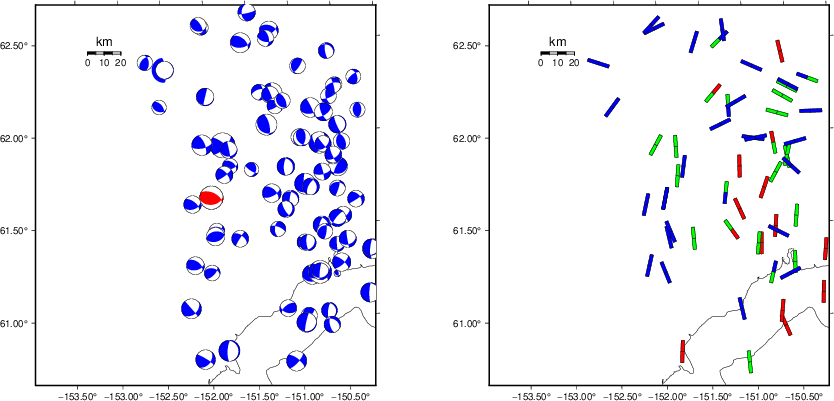
Context
The left panel of the next figure presents the focal mechanism for this earthquake (red) in the context of other nearby events (blue) in the SLU Moment Tensor Catalog. The right panel shows the inferred direction of maximum compressive stress and the type of faulting (green is strike-slip, red is normal, blue is thrust; oblique is shown by a combination of colors). Thus context plot is useful for assessing the appropriateness of the moment tensor of this event.
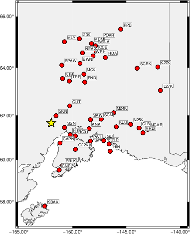
Waveform Inversion using wvfgrd96
The focal mechanism was determined using broadband seismic waveforms. The location of the event (star) and the
stations used for (red) the waveform inversion are shown in the next figure.
|
|
Location of broadband stations used for waveform inversion
|
The program wvfgrd96 was used with good traces observed at short distance to determine the focal mechanism, depth and seismic moment. This technique requires a high quality signal and well determined velocity model for the Green's functions. To the extent that these are the quality data, this type of mechanism should be preferred over the radiation pattern technique which requires the separate step of defining the pressure and tension quadrants and the correct strike.
The observed and predicted traces are filtered using the following gsac commands:
cut o DIST/3.3 -30 o DIST/3.3 +70
rtr
taper w 0.1
hp c 0.02 n 3
lp c 0.06 n 3
The results of this grid search are as follow:
           DEPTH  STK   DIP  RAKE   MW    FIT
WVFGRD96    2.0    45    45   -85   5.00 0.1493
WVFGRD96    4.0    60    80    40   5.05 0.1530
WVFGRD96    6.0    60    80    40   5.10 0.1867
WVFGRD96    8.0    55    90    50   5.17 0.2093
WVFGRD96   10.0    55    90    45   5.18 0.2282
WVFGRD96   12.0    55    90    45   5.20 0.2374
WVFGRD96   14.0    60    80    40   5.21 0.2424
WVFGRD96   16.0    60    80    40   5.23 0.2451
WVFGRD96   18.0    60    80    40   5.24 0.2461
WVFGRD96   20.0    60    80    40   5.25 0.2461
WVFGRD96   22.0    60    80    40   5.27 0.2458
WVFGRD96   24.0    60    80    40   5.28 0.2448
WVFGRD96   26.0    60    80    40   5.29 0.2428
WVFGRD96   28.0    60    80    40   5.31 0.2399
WVFGRD96   30.0    60    80    35   5.32 0.2363
WVFGRD96   32.0    60    80    35   5.34 0.2321
WVFGRD96   34.0    60    85    35   5.35 0.2286
WVFGRD96   36.0   240    90   -30   5.37 0.2236
WVFGRD96   38.0   240    90   -30   5.39 0.2231
WVFGRD96   40.0    65    85    40   5.48 0.2254
WVFGRD96   42.0    55    65   -30   5.55 0.2285
WVFGRD96   44.0    55    65   -30   5.57 0.2313
WVFGRD96   46.0    55    65   -30   5.58 0.2333
WVFGRD96   48.0    55    60   -25   5.59 0.2348
WVFGRD96   50.0    55    60   -25   5.60 0.2382
WVFGRD96   52.0    55    60   -25   5.62 0.2415
WVFGRD96   54.0    55    55     0   5.60 0.2484
WVFGRD96   56.0    55    55     0   5.61 0.2581
WVFGRD96   58.0    60    55    15   5.61 0.2697
WVFGRD96   60.0    60    55    15   5.63 0.2821
WVFGRD96   62.0    60    55    15   5.64 0.2943
WVFGRD96   64.0    60    55    15   5.65 0.3055
WVFGRD96   66.0    65    55    20   5.67 0.3159
WVFGRD96   68.0    65    55    20   5.68 0.3249
WVFGRD96   70.0    65    55    20   5.69 0.3372
WVFGRD96   72.0    65    55    20   5.70 0.3496
WVFGRD96   74.0    65    50    20   5.71 0.3603
WVFGRD96   76.0    70    45    40   5.70 0.3700
WVFGRD96   78.0    70    45    40   5.71 0.3822
WVFGRD96   80.0    70    45    45   5.72 0.3925
WVFGRD96   82.0    70    45    45   5.73 0.4022
WVFGRD96   84.0    70    45    45   5.73 0.4117
WVFGRD96   86.0    75    40    50   5.74 0.4210
WVFGRD96   88.0    80    40    55   5.75 0.4297
WVFGRD96   90.0    80    40    55   5.76 0.4386
WVFGRD96   92.0    80    40    55   5.76 0.4466
WVFGRD96   94.0    80    40    55   5.77 0.4539
WVFGRD96   96.0    80    40    55   5.78 0.4606
WVFGRD96   98.0    80    40    55   5.78 0.4668
WVFGRD96  100.0    80    40    55   5.79 0.4726
WVFGRD96  102.0    80    40    55   5.79 0.4775
WVFGRD96  104.0    80    40    60   5.79 0.4821
WVFGRD96  106.0    80    40    60   5.80 0.4862
WVFGRD96  108.0    80    40    60   5.80 0.4896
WVFGRD96  110.0    80    40    60   5.80 0.4923
WVFGRD96  112.0    80    40    60   5.81 0.4948
WVFGRD96  114.0    80    40    60   5.81 0.4964
WVFGRD96  116.0    85    40    65   5.82 0.4977
WVFGRD96  118.0    85    40    65   5.82 0.4991
WVFGRD96  120.0    85    40    65   5.82 0.4997
WVFGRD96  122.0    85    40    65   5.82 0.5001
WVFGRD96  124.0    85    40    65   5.83 0.4994
WVFGRD96  126.0    85    40    65   5.83 0.4984
WVFGRD96  128.0    85    40    65   5.83 0.4976
The best solution is
WVFGRD96 122.0 85 40 65 5.82 0.5001
The mechanism corresponding to the best fit is
|
|
Figure 1. Waveform inversion focal mechanism
|
The best fit as a function of depth is given in the following figure:
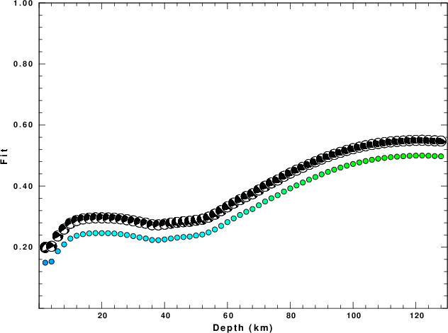
|
|
Figure 2. Depth sensitivity for waveform mechanism
|
The comparison of the observed and predicted waveforms is given in the next figure. The red traces are the observed and the blue are the predicted.
Each observed-predicted component is plotted to the same scale and peak amplitudes are indicated by the numbers to the left of each trace. A pair of numbers is given in black at the right of each predicted traces. The upper number it the time shift required for maximum correlation between the observed and predicted traces. This time shift is required because the synthetics are not computed at exactly the same distance as the observed, the velocity model used in the predictions may not be perfect and the epicentral parameters may be be off.
A positive time shift indicates that the prediction is too fast and should be delayed to match the observed trace (shift to the right in this figure). A negative value indicates that the prediction is too slow. The lower number gives the percentage of variance reduction to characterize the individual goodness of fit (100% indicates a perfect fit).
The bandpass filter used in the processing and for the display was
cut o DIST/3.3 -30 o DIST/3.3 +70
rtr
taper w 0.1
hp c 0.02 n 3
lp c 0.06 n 3
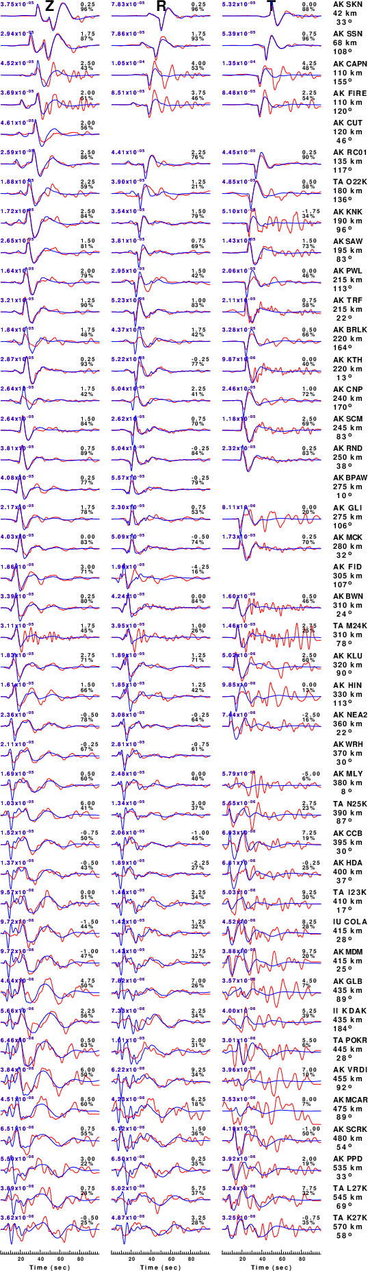
|
|
Figure 3. Waveform comparison for selected depth. Red: observed; Blue - predicted. The time shift with respect to the model prediction is indicated. The percent of fit is also indicated. The time scale is relative to the first trace sample.
|
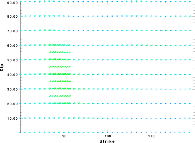
|
|
Focal mechanism sensitivity at the preferred depth. The red color indicates a very good fit to the waveforms.
Each solution is plotted as a vector at a given value of strike and dip with the angle of the vector representing the rake angle, measured, with respect to the upward vertical (N) in the figure.
|
A check on the assumed source location is possible by looking at the time shifts between the observed and predicted traces. The time shifts for waveform matching arise for several reasons:
- The origin time and epicentral distance are incorrect
- The velocity model used for the inversion is incorrect
- The velocity model used to define the P-arrival time is not the
same as the velocity model used for the waveform inversion
(assuming that the initial trace alignment is based on the
P arrival time)
Assuming only a mislocation, the time shifts are fit to a functional form:
Time_shift = A + B cos Azimuth + C Sin Azimuth
The time shifts for this inversion lead to the next figure:
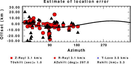
The derived shift in origin time and epicentral coordinates are given at the bottom of the figure.
Velocity Model
The WUS.model used for the waveform synthetic seismograms and for the surface wave eigenfunctions and dispersion is as follows
(The format is in the model96 format of Computer Programs in Seismology).
MODEL.01
Model after     8 iterations
ISOTROPIC
KGS
FLAT EARTH
1-D
CONSTANT VELOCITY
LINE08
LINE09
LINE10
LINE11
      H(KM)   VP(KM/S)   VS(KM/S) RHO(GM/CC)         QP         QS       ETAP       ETAS      FREFP      FREFS
     1.9000     3.4065     2.0089     2.2150  0.302E-02  0.679E-02   0.00       0.00       1.00       1.00
     6.1000     5.5445     3.2953     2.6089  0.349E-02  0.784E-02   0.00       0.00       1.00       1.00
    13.0000     6.2708     3.7396     2.7812  0.212E-02  0.476E-02   0.00       0.00       1.00       1.00
    19.0000     6.4075     3.7680     2.8223  0.111E-02  0.249E-02   0.00       0.00       1.00       1.00
     0.0000     7.9000     4.6200     3.2760  0.164E-10  0.370E-10   0.00       0.00       1.00       1.00
Last Changed Fri Apr 26 06:28:53 PM CDT 2024