Location

Location ANSS

The ANSS event ID is ak0157mvsl0s and the event page is at https://earthquake.usgs.gov/earthquakes/eventpage/ak0157mvsl0s/executive.

2015/06/15 21:13:40 63.239 -150.622 129.8 4 Alaska

Focal Mechanism

USGS/SLU Moment Tensor Solution ENS 2015/06/15 21:13:40:0 63.24 -150.62 129.8 4.0 Alaska Stations used: AK.CCB AK.CUT AK.DOT AK.FIRE AK.GHO AK.GLI AK.HDA AK.HIN AK.KLU AK.KNK AK.KTH AK.MCK AK.MDM AK.MLY AK.NEA2 AK.PAX AK.PWL AK.RC01 AK.RND AK.SAW AK.SCM AK.SKN AK.SSN AK.TRF AK.WAT3 AK.WAT4 AK.WRH AT.PMR AT.TTA IM.IL31 IU.COLA TA.I23K TA.POKR TA.TCOL Filtering commands used: cut a -20 a 100 rtr taper w 0.1 hp c 0.02 n 3 lp c 0.10 n 3 Best Fitting Double Couple Mo = 1.30e+22 dyne-cm Mw = 4.01 Z = 110 km Plane Strike Dip Rake NP1 40 75 60 NP2 286 33 152 Principal Axes: Axis Value Plunge Azimuth T 1.30e+22 51 276 N 0.00e+00 29 49 P -1.30e+22 24 153 Moment Tensor: (dyne-cm) Component Value Mxx -8.53e+21 Mxy 3.87e+21 Mxz 4.99e+21 Myy 2.89e+21 Myz -8.57e+21 Mzz 5.64e+21 -------------- ---------------------- ---------------------------# --------#########-----------## ----#####################----##### --################################## -############################---###### -############################------##### ############################--------#### ########## ###############-----------### ########## T ##############------------### ########## ############---------------## ########################-----------------# #####################------------------- ###################--------------------- ################---------------------- #############----------------------- ##########------------- -------- ######--------------- P ------ #------------------- ----- ---------------------- -------------- Global CMT Convention Moment Tensor: R T P 5.64e+21 4.99e+21 8.57e+21 4.99e+21 -8.53e+21 -3.87e+21 8.57e+21 -3.87e+21 2.89e+21 Details of the solution is found at http://www.eas.slu.edu/eqc/eqc_mt/MECH.NA/20150615211340/index.html

Preferred Solution

The preferred solution from an analysis of the surface-wave spectral amplitude radiation pattern, waveform inversion or first motion observations is

      STK = 40
      DIP = 75
     RAKE = 60
       MW = 4.01
       HS = 110.0

The NDK file is 20150615211340.ndk The waveform inversion is preferred.

Magnitudes

Given the availability of digital waveforms for determination of the moment tensor, this section documents the added processing leading to mLg, if appropriate to the region, and M_L by application of the respective IASPEI formulae. As a research study, the linear distance term of the IASPEI formula for M_L is adjusted to remove a linear distance trend in residuals to give a regionally defined M_L. The defined M_L uses horizontal component recordings, but the same procedure is applied to the vertical components since there may be some interest in vertical component ground motions. Residual plots versus distance may indicate interesting features of ground motion scaling in some distance ranges. A residual plot of the regionalized magnitude is given as a function of distance and azimuth, since data sets may transcend different wave propagation provinces.

ML Magnitude

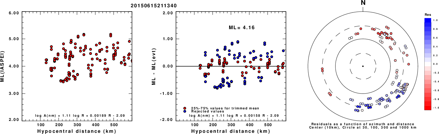
Left: ML computed using the IASPEI formula for Horizontal components. Center: ML residuals computed using a modified IASPEI formula that accounts for path specific attenuation; the values used for the trimmed mean are indicated. The ML relation used for each figure is given at the bottom of each plot. Right: Residuals from new relation as a function of distance and azimuth.

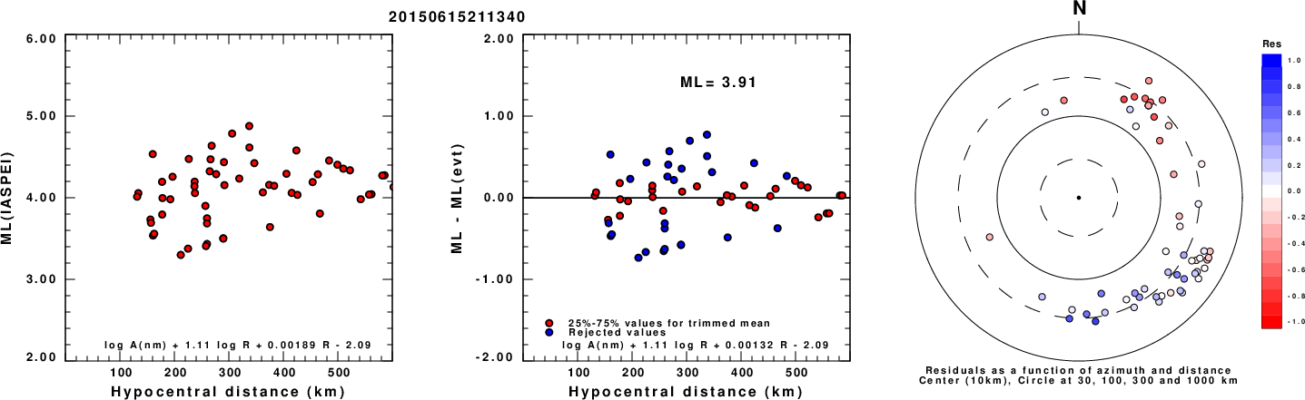
Left: ML computed using the IASPEI formula for Vertical components (research). Center: ML residuals computed using a modified IASPEI formula that accounts for path specific attenuation; the values used for the trimmed mean are indicated. The ML relation used for each figure is given at the bottom of each plot. Right: Residuals from new relation as a function of distance and azimuth.

Context

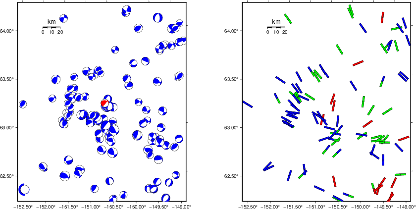
The left panel of the next figure presents the focal mechanism for this earthquake (red) in the context of other nearby events (blue) in the SLU Moment Tensor Catalog. The right panel shows the inferred direction of maximum compressive stress and the type of faulting (green is strike-slip, red is normal, blue is thrust; oblique is shown by a combination of colors). Thus context plot is useful for assessing the appropriateness of the moment tensor of this event.

Waveform Inversion using wvfgrd96

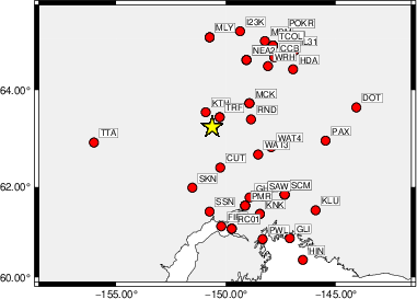
The focal mechanism was determined using broadband seismic waveforms. The location of the event (star) and the stations used for (red) the waveform inversion are shown in the next figure.

Location of broadband stations used for waveform inversion

The program wvfgrd96 was used with good traces observed at short distance to determine the focal mechanism, depth and seismic moment. This technique requires a high quality signal and well determined velocity model for the Green's functions. To the extent that these are the quality data, this type of mechanism should be preferred over the radiation pattern technique which requires the separate step of defining the pressure and tension quadrants and the correct strike.

The observed and predicted traces are filtered using the following gsac commands:

cut a -20 a 100
rtr
taper w 0.1
hp c 0.02 n 3 
lp c 0.10 n 3

The results of this grid search are as follow:

           DEPTH  STK   DIP  RAKE   MW    FIT
WVFGRD96   50.0   215    75   -40   3.83 0.3119
WVFGRD96   52.0   210    75   -30   3.85 0.3263
WVFGRD96   54.0   210    75   -30   3.87 0.3441
WVFGRD96   56.0   210    80   -30   3.88 0.3600
WVFGRD96   58.0   210    80   -30   3.90 0.3757
WVFGRD96   60.0    35    85    30   3.90 0.3909
WVFGRD96   62.0    35    85    30   3.91 0.4060
WVFGRD96   64.0    35    85    35   3.92 0.4191
WVFGRD96   66.0    35    80    35   3.93 0.4306
WVFGRD96   68.0    35    80    35   3.94 0.4418
WVFGRD96   70.0    35    80    35   3.94 0.4517
WVFGRD96   72.0    35    80    35   3.95 0.4587
WVFGRD96   74.0    35    80    40   3.95 0.4661
WVFGRD96   76.0    35    80    40   3.95 0.4719
WVFGRD96   78.0    35    80    40   3.96 0.4802
WVFGRD96   80.0    35    80    40   3.96 0.4885
WVFGRD96   82.0    35    80    45   3.97 0.4968
WVFGRD96   84.0    35    80    45   3.97 0.5044
WVFGRD96   86.0    35    80    45   3.98 0.5103
WVFGRD96   88.0    35    80    50   3.98 0.5176
WVFGRD96   90.0    35    80    50   3.98 0.5224
WVFGRD96   92.0    35    80    50   3.99 0.5284
WVFGRD96   94.0    40    75    55   3.98 0.5334
WVFGRD96   96.0    40    75    55   3.99 0.5372
WVFGRD96   98.0    40    75    55   3.99 0.5428
WVFGRD96  100.0    40    75    55   3.99 0.5463
WVFGRD96  102.0    40    75    55   4.00 0.5471
WVFGRD96  104.0    40    75    60   4.00 0.5505
WVFGRD96  106.0    40    75    60   4.00 0.5513
WVFGRD96  108.0    40    75    60   4.01 0.5528
WVFGRD96  110.0    40    75    60   4.01 0.5543
WVFGRD96  112.0    40    75    60   4.01 0.5537
WVFGRD96  114.0    40    75    60   4.01 0.5536
WVFGRD96  116.0    40    75    65   4.02 0.5533
WVFGRD96  118.0    40    75    65   4.02 0.5538
WVFGRD96  120.0    40    75    65   4.02 0.5535
WVFGRD96  122.0    40    75    65   4.02 0.5530
WVFGRD96  124.0    40    75    65   4.02 0.5509
WVFGRD96  126.0    40    75    65   4.03 0.5504
WVFGRD96  128.0    40    75    65   4.03 0.5502
WVFGRD96  130.0    40    75    65   4.03 0.5477
WVFGRD96  132.0    40    75    65   4.03 0.5464
WVFGRD96  134.0    40    75    70   4.04 0.5463
WVFGRD96  136.0    40    75    70   4.04 0.5436
WVFGRD96  138.0    40    75    70   4.04 0.5417

The best solution is

WVFGRD96  110.0    40    75    60   4.01 0.5543

The mechanism corresponding to the best fit is

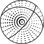
Figure 1. Waveform inversion focal mechanism

The best fit as a function of depth is given in the following figure:

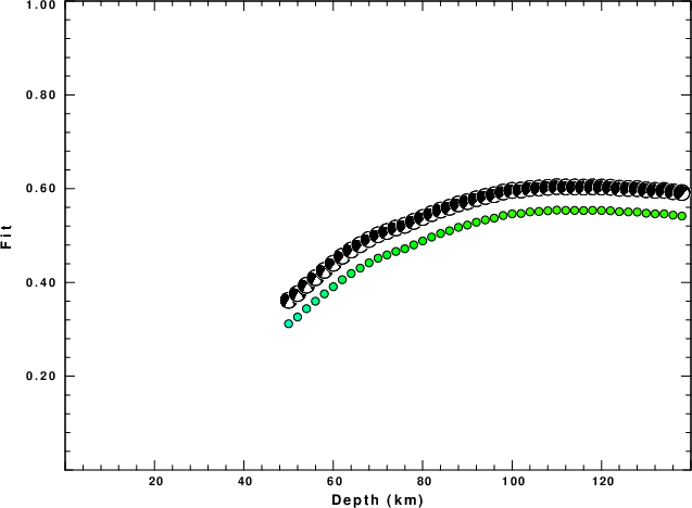
Figure 2. Depth sensitivity for waveform mechanism

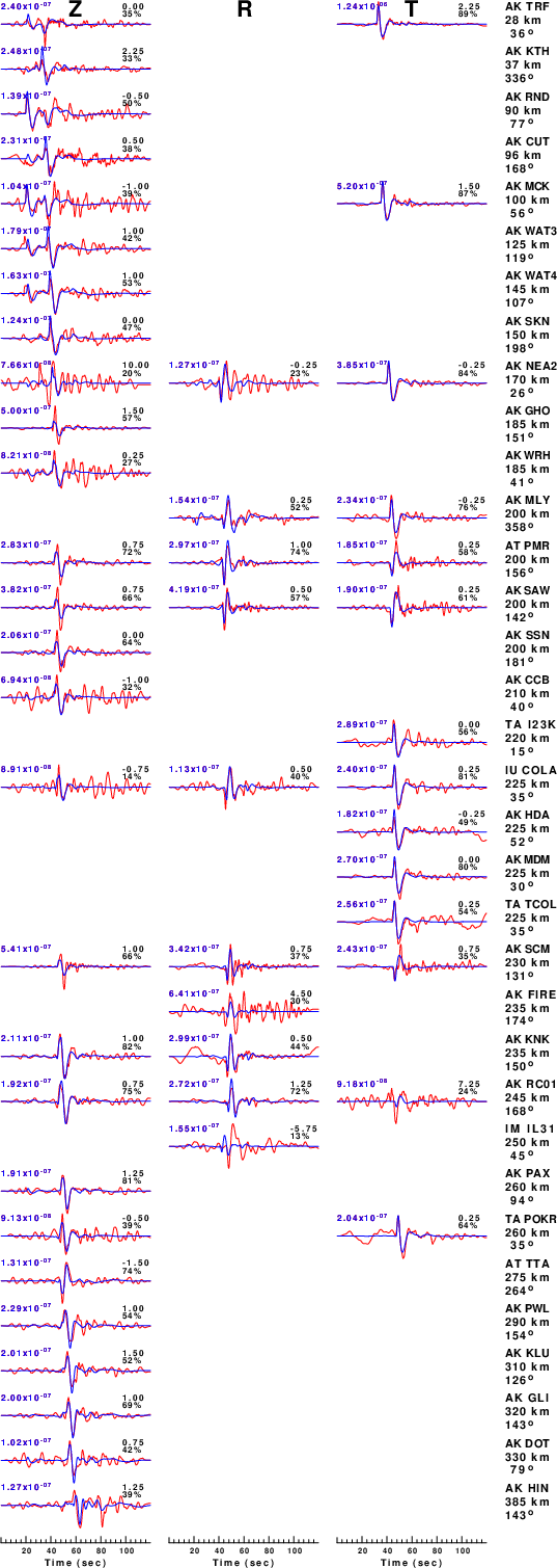
The comparison of the observed and predicted waveforms is given in the next figure. The red traces are the observed and the blue are the predicted. Each observed-predicted component is plotted to the same scale and peak amplitudes are indicated by the numbers to the left of each trace. A pair of numbers is given in black at the right of each predicted traces. The upper number it the time shift required for maximum correlation between the observed and predicted traces. This time shift is required because the synthetics are not computed at exactly the same distance as the observed, the velocity model used in the predictions may not be perfect and the epicentral parameters may be be off. A positive time shift indicates that the prediction is too fast and should be delayed to match the observed trace (shift to the right in this figure). A negative value indicates that the prediction is too slow. The lower number gives the percentage of variance reduction to characterize the individual goodness of fit (100% indicates a perfect fit).

The bandpass filter used in the processing and for the display was

cut a -20 a 100
rtr
taper w 0.1
hp c 0.02 n 3 
lp c 0.10 n 3

Figure 3. Waveform comparison for selected depth. Red: observed; Blue - predicted. The time shift with respect to the model prediction is indicated. The percent of fit is also indicated. The time scale is relative to the first trace sample.

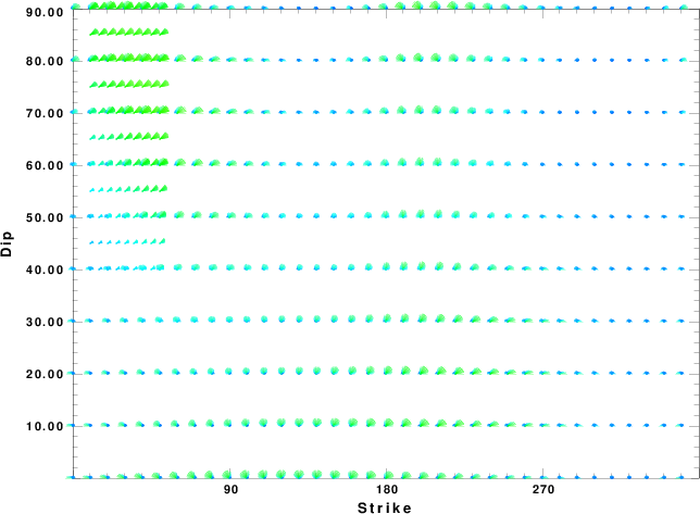
Focal mechanism sensitivity at the preferred depth. The red color indicates a very good fit to the waveforms. Each solution is plotted as a vector at a given value of strike and dip with the angle of the vector representing the rake angle, measured, with respect to the upward vertical (N) in the figure.

A check on the assumed source location is possible by looking at the time shifts between the observed and predicted traces. The time shifts for waveform matching arise for several reasons:

The origin time and epicentral distance are incorrect
The velocity model used for the inversion is incorrect
The velocity model used to define the P-arrival time is not the same as the velocity model used for the waveform inversion (assuming that the initial trace alignment is based on the P arrival time)

Assuming only a mislocation, the time shifts are fit to a functional form:

 Time_shift = A + B cos Azimuth + C Sin Azimuth

The time shifts for this inversion lead to the next figure:

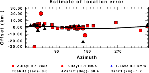
The derived shift in origin time and epicentral coordinates are given at the bottom of the figure.

Velocity Model

The WUS.model used for the waveform synthetic seismograms and for the surface wave eigenfunctions and dispersion is as follows (The format is in the model96 format of Computer Programs in Seismology).

MODEL.01
Model after     8 iterations
ISOTROPIC
KGS
FLAT EARTH
1-D
CONSTANT VELOCITY
LINE08
LINE09
LINE10
LINE11
      H(KM)   VP(KM/S)   VS(KM/S) RHO(GM/CC)         QP         QS       ETAP       ETAS      FREFP      FREFS
     1.9000     3.4065     2.0089     2.2150  0.302E-02  0.679E-02   0.00       0.00       1.00       1.00    
     6.1000     5.5445     3.2953     2.6089  0.349E-02  0.784E-02   0.00       0.00       1.00       1.00    
    13.0000     6.2708     3.7396     2.7812  0.212E-02  0.476E-02   0.00       0.00       1.00       1.00    
    19.0000     6.4075     3.7680     2.8223  0.111E-02  0.249E-02   0.00       0.00       1.00       1.00    
     0.0000     7.9000     4.6200     3.2760  0.164E-10  0.370E-10   0.00       0.00       1.00       1.00

Last Changed Fri Apr 26 05:49:59 PM CDT 2024