Location
Location ANSS
The ANSS event ID is us20002avh and the event page is at
https://earthquake.usgs.gov/earthquakes/eventpage/us20002avh/executive.
2015/05/02 16:23:07 42.236 -85.428 4.5 4.2 Michigan
Focal Mechanism
 USGS/SLU Moment Tensor Solution
 ENS  2015/05/02 16:23:07:0  42.24  -85.43   4.5 4.2 Michigan

 Stations used:
   CN.SADO IU.WCI LD.ALLY LD.WVNY N4.D41A N4.E43A N4.E46A
   N4.F42A N4.G40A N4.G45A N4.H43A N4.I40B N4.I42A N4.I45A
   N4.I49A N4.J47A N4.J54A N4.K43A N4.K50A N4.L40A N4.L42A
   N4.L48A N4.M44A N4.M50A N4.M52A N4.N41A N4.N47A N4.N49A
   N4.N51A N4.N53A N4.O44A N4.O49A N4.O52A N4.O54A N4.P43A
   N4.P46A N4.P48A N4.P51A N4.P53A N4.Q44B N4.Q51A N4.Q52A
   N4.Q54A N4.R49A N4.R50A N4.R53A N4.S44A N4.S51A N4.T47A
   N4.T50A NM.BLO NM.SIUC NM.SLM NM.USIN NW.HQIL TA.L44A
   TA.M53A TA.M54A TA.N54A TA.O53A TA.P49A TA.P52A TA.SFIN
   US.AAM US.ACSO US.COWI US.ERPA US.GLMI US.HDIL US.JFWS
   WU.MEDO

 Filtering commands used:
   cut o DIST/3.3 -30 o DIST/3.3 +70
   rtr
   taper w 0.1
   hp c 0.03 n 3
   lp c 0.10 n 3

 Best Fitting Double Couple
  Mo = 2.88e+22 dyne-cm
  Mw = 4.24
  Z  = 5 km
  Plane   Strike  Dip  Rake
   NP1      210    90   -175
   NP2      120    85     0
  Principal Axes:
   Axis    Value   Plunge  Azimuth
    T   2.88e+22      4     345
    N   0.00e+00     85     210
    P  -2.88e+22      4      75

 Moment Tensor: (dyne-cm)
    Component   Value
       Mxx     2.49e+22
       Mxy    -1.44e+22
       Mxz     1.26e+21
       Myy    -2.49e+22
       Myz    -2.18e+21
       Mzz     0.00e+00


                      T ###########
                 ####   ##############-
              #######################-----
             #######################-------
           ########################----------
          ########################------------
         ----####################--------------
        -------#################--------------
        ----------#############--------------- P
       --------------#########----------------
       -----------------#####--------------------
       ------------------------------------------
       -------------------####-------------------
        -----------------#########--------------
        ----------------#############-----------
         --------------##################------
          ------------#######################-
           ----------########################
             -------#######################
              -----#######################
                 -#####################
                     ##############


 Global CMT Convention Moment Tensor:
      R          T          P
  0.00e+00   1.26e+21   2.18e+21
  1.26e+21   2.49e+22   1.44e+22
  2.18e+21   1.44e+22  -2.49e+22


Details of the solution is found at

http://www.eas.slu.edu/eqc/eqc_mt/MECH.NA/20150502162307/index.html
|
Preferred Solution
The preferred solution from an analysis of the surface-wave spectral amplitude radiation pattern, waveform inversion or first motion observations is
      STK = 120
      DIP = 85
     RAKE = 0
       MW = 4.24
       HS = 5.0
The NDK file is 20150502162307.ndk
The waveform inversion is preferred.
Moment Tensor Comparison
The following compares this source inversion to those provided by others. The purpose is to look for major differences and also to note slight differences that might be inherent to the processing procedure. For completeness the USGS/SLU solution is repeated from above.
| SLU |
USGSMT |
 USGS/SLU Moment Tensor Solution
 ENS  2015/05/02 16:23:07:0  42.24  -85.43   4.5 4.2 Michigan

 Stations used:
   CN.SADO IU.WCI LD.ALLY LD.WVNY N4.D41A N4.E43A N4.E46A
   N4.F42A N4.G40A N4.G45A N4.H43A N4.I40B N4.I42A N4.I45A
   N4.I49A N4.J47A N4.J54A N4.K43A N4.K50A N4.L40A N4.L42A
   N4.L48A N4.M44A N4.M50A N4.M52A N4.N41A N4.N47A N4.N49A
   N4.N51A N4.N53A N4.O44A N4.O49A N4.O52A N4.O54A N4.P43A
   N4.P46A N4.P48A N4.P51A N4.P53A N4.Q44B N4.Q51A N4.Q52A
   N4.Q54A N4.R49A N4.R50A N4.R53A N4.S44A N4.S51A N4.T47A
   N4.T50A NM.BLO NM.SIUC NM.SLM NM.USIN NW.HQIL TA.L44A
   TA.M53A TA.M54A TA.N54A TA.O53A TA.P49A TA.P52A TA.SFIN
   US.AAM US.ACSO US.COWI US.ERPA US.GLMI US.HDIL US.JFWS
   WU.MEDO

 Filtering commands used:
   cut o DIST/3.3 -30 o DIST/3.3 +70
   rtr
   taper w 0.1
   hp c 0.03 n 3
   lp c 0.10 n 3

 Best Fitting Double Couple
  Mo = 2.88e+22 dyne-cm
  Mw = 4.24
  Z  = 5 km
  Plane   Strike  Dip  Rake
   NP1      210    90   -175
   NP2      120    85     0
  Principal Axes:
   Axis    Value   Plunge  Azimuth
    T   2.88e+22      4     345
    N   0.00e+00     85     210
    P  -2.88e+22      4      75

 Moment Tensor: (dyne-cm)
    Component   Value
       Mxx     2.49e+22
       Mxy    -1.44e+22
       Mxz     1.26e+21
       Myy    -2.49e+22
       Myz    -2.18e+21
       Mzz     0.00e+00


                      T ###########
                 ####   ##############-
              #######################-----
             #######################-------
           ########################----------
          ########################------------
         ----####################--------------
        -------#################--------------
        ----------#############--------------- P
       --------------#########----------------
       -----------------#####--------------------
       ------------------------------------------
       -------------------####-------------------
        -----------------#########--------------
        ----------------#############-----------
         --------------##################------
          ------------#######################-
           ----------########################
             -------#######################
              -----#######################
                 -#####################
                     ##############


 Global CMT Convention Moment Tensor:
      R          T          P
  0.00e+00   1.26e+21   2.18e+21
  1.26e+21   2.49e+22   1.44e+22
  2.18e+21   1.44e+22  -2.49e+22


Details of the solution is found at

http://www.eas.slu.edu/eqc/eqc_mt/MECH.NA/20150502162307/index.html
|
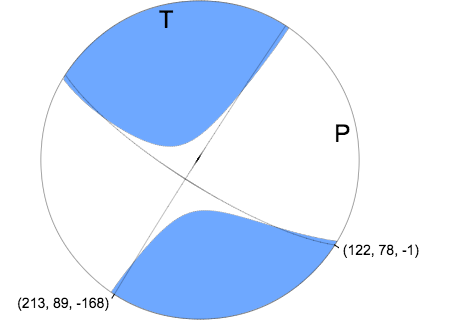
Regional Moment Tensor (Mwr)
Moment	2.139e+15 N-m
Magnitude	4.15
Depth	8.0 km
Percent DC	80%
Half Duration	–
Catalog	US (us20002avh)
Data Source	US1
Contributor	US1
Nodal Planes
Plane	Strike	Dip	Rake
NP1	213	89	-168
NP2	122	78	-1
Principal Axes
Axis	Value	Plunge	Azimuth
T	2.241	8	347
N	-0.222	78	218
P	-2.020	9	78
|
Magnitudes
Given the availability of digital waveforms for determination of the moment tensor, this section documents the added processing leading to mLg, if appropriate to the region, and ML by application of the respective IASPEI formulae. As a research study, the linear distance term of the IASPEI formula
for ML is adjusted to remove a linear distance trend in residuals to give a regionally defined ML. The defined ML uses horizontal component recordings, but the same procedure is applied to the vertical components since there may be some interest in vertical component ground motions. Residual plots versus distance may indicate interesting features of ground motion scaling in some distance ranges. A residual plot of the regionalized magnitude is given as a function of distance and azimuth, since data sets may transcend different wave propagation provinces.
mLg Magnitude
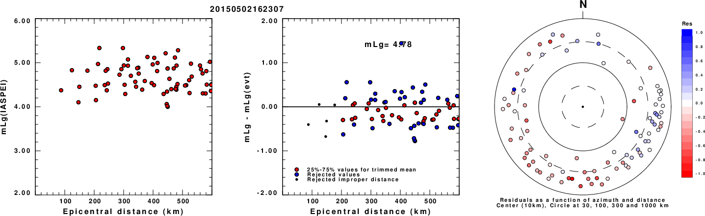
Left: mLg computed using the IASPEI formula. Center: mLg residuals versus epicentral distance ; the values used for the trimmed mean magnitude estimate are indicated.
Right: residuals as a function of distance and azimuth.
ML Magnitude
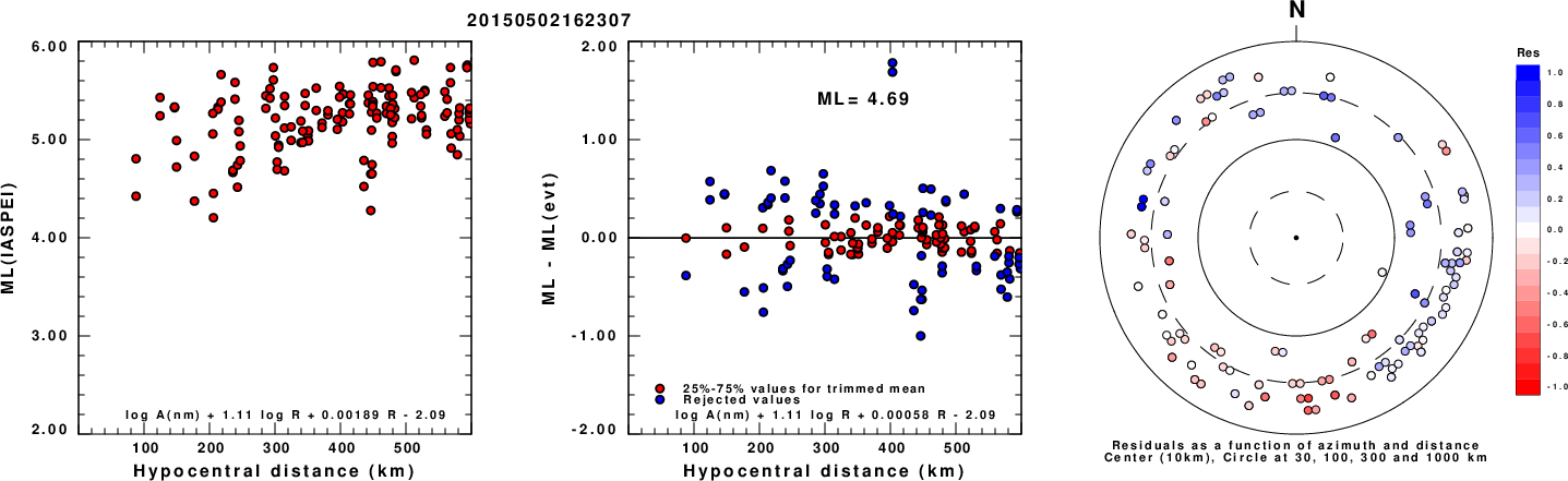
Left: ML computed using the IASPEI formula for Horizontal components. Center: ML residuals computed using a modified IASPEI formula that accounts for path specific attenuation; the values used for the trimmed mean are indicated. The ML relation used for each figure is given at the bottom of each plot.
Right: Residuals from new relation as a function of distance and azimuth.
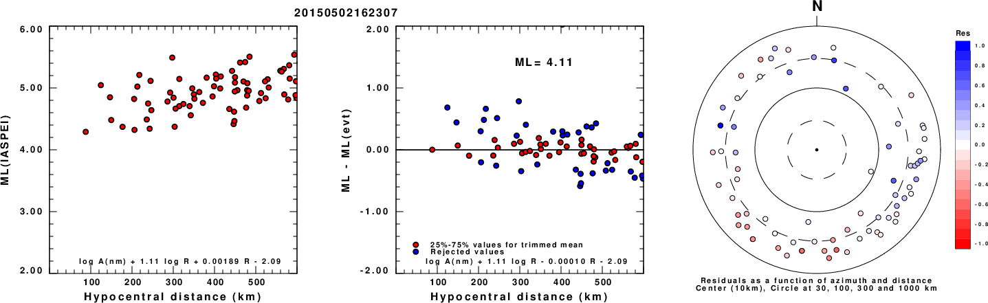
Left: ML computed using the IASPEI formula for Vertical components (research). Center: ML residuals computed using a modified IASPEI formula that accounts for path specific attenuation; the values used for the trimmed mean are indicated. The ML relation used for each figure is given at the bottom of each plot.
Right: Residuals from new relation as a function of distance and azimuth.
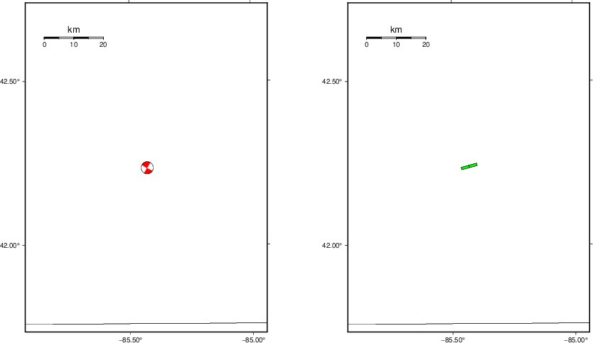
Context
The left panel of the next figure presents the focal mechanism for this earthquake (red) in the context of other nearby events (blue) in the SLU Moment Tensor Catalog. The right panel shows the inferred direction of maximum compressive stress and the type of faulting (green is strike-slip, red is normal, blue is thrust; oblique is shown by a combination of colors). Thus context plot is useful for assessing the appropriateness of the moment tensor of this event.
Waveform Inversion using wvfgrd96
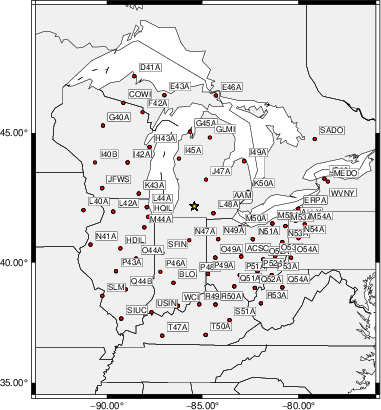
The focal mechanism was determined using broadband seismic waveforms. The location of the event (star) and the
stations used for (red) the waveform inversion are shown in the next figure.
|
|
Location of broadband stations used for waveform inversion
|
The program wvfgrd96 was used with good traces observed at short distance to determine the focal mechanism, depth and seismic moment. This technique requires a high quality signal and well determined velocity model for the Green's functions. To the extent that these are the quality data, this type of mechanism should be preferred over the radiation pattern technique which requires the separate step of defining the pressure and tension quadrants and the correct strike.
The observed and predicted traces are filtered using the following gsac commands:
cut o DIST/3.3 -30 o DIST/3.3 +70
rtr
taper w 0.1
hp c 0.03 n 3
lp c 0.10 n 3
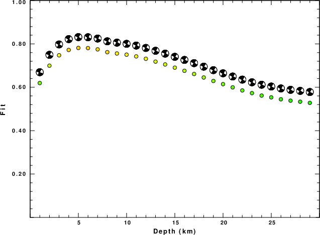
The results of this grid search are as follow:
           DEPTH  STK   DIP  RAKE   MW    FIT
WVFGRD96    1.0   115    80    -5   4.13 0.6195
WVFGRD96    2.0   115    85     0   4.17 0.6996
WVFGRD96    3.0   120    85     0   4.20 0.7475
WVFGRD96    4.0   120    85     0   4.23 0.7721
WVFGRD96    5.0   120    85     0   4.24 0.7813
WVFGRD96    6.0   120    85     0   4.25 0.7807
WVFGRD96    7.0   120    85     0   4.26 0.7748
WVFGRD96    8.0   300    90    -5   4.27 0.7619
WVFGRD96    9.0   300    85     5   4.28 0.7558
WVFGRD96   10.0   120    85     5   4.29 0.7503
WVFGRD96   11.0   300    85     0   4.30 0.7424
WVFGRD96   12.0   300    85     5   4.31 0.7314
WVFGRD96   13.0   120    90     0   4.32 0.7183
WVFGRD96   14.0   300    85     0   4.32 0.7052
WVFGRD96   15.0   300    90     0   4.33 0.6905
WVFGRD96   16.0   120    90     0   4.33 0.6761
WVFGRD96   17.0   300    90     0   4.34 0.6613
WVFGRD96   18.0   120    90     0   4.35 0.6452
WVFGRD96   19.0   120    90     5   4.36 0.6290
WVFGRD96   20.0   120    85     5   4.36 0.6145
WVFGRD96   21.0   120    90     5   4.37 0.5997
WVFGRD96   22.0   120    85     5   4.37 0.5854
WVFGRD96   23.0   120    85     0   4.38 0.5731
WVFGRD96   24.0   300    90     0   4.38 0.5618
WVFGRD96   25.0   120    85     0   4.39 0.5535
WVFGRD96   26.0   120    85     0   4.39 0.5447
WVFGRD96   27.0   120    85    -5   4.40 0.5383
WVFGRD96   28.0   120    85    -5   4.40 0.5335
WVFGRD96   29.0   120    85    -5   4.41 0.5282
The best solution is
WVFGRD96 5.0 120 85 0 4.24 0.7813
The mechanism corresponding to the best fit is
|
|
Figure 1. Waveform inversion focal mechanism
|
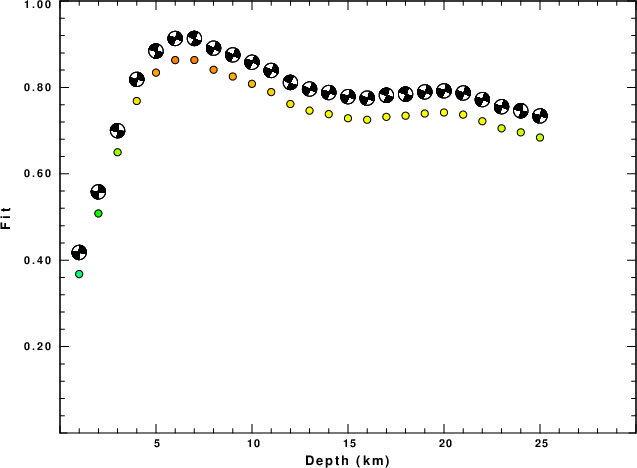
The best fit as a function of depth is given in the following figure:
|
|
Figure 2. Depth sensitivity for waveform mechanism
|
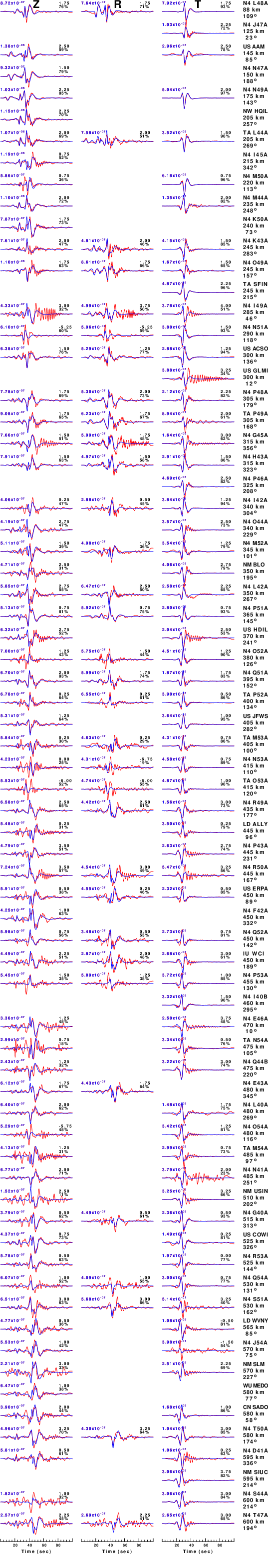
The comparison of the observed and predicted waveforms is given in the next figure. The red traces are the observed and the blue are the predicted.
Each observed-predicted component is plotted to the same scale and peak amplitudes are indicated by the numbers to the left of each trace. A pair of numbers is given in black at the right of each predicted traces. The upper number it the time shift required for maximum correlation between the observed and predicted traces. This time shift is required because the synthetics are not computed at exactly the same distance as the observed, the velocity model used in the predictions may not be perfect and the epicentral parameters may be be off.
A positive time shift indicates that the prediction is too fast and should be delayed to match the observed trace (shift to the right in this figure). A negative value indicates that the prediction is too slow. The lower number gives the percentage of variance reduction to characterize the individual goodness of fit (100% indicates a perfect fit).
The bandpass filter used in the processing and for the display was
cut o DIST/3.3 -30 o DIST/3.3 +70
rtr
taper w 0.1
hp c 0.03 n 3
lp c 0.10 n 3
|
|
Figure 3. Waveform comparison for selected depth. Red: observed; Blue - predicted. The time shift with respect to the model prediction is indicated. The percent of fit is also indicated. The time scale is relative to the first trace sample.
|
|
|
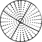
Focal mechanism sensitivity at the preferred depth. The red color indicates a very good fit to the waveforms.
Each solution is plotted as a vector at a given value of strike and dip with the angle of the vector representing the rake angle, measured, with respect to the upward vertical (N) in the figure.
|
A check on the assumed source location is possible by looking at the time shifts between the observed and predicted traces. The time shifts for waveform matching arise for several reasons:
- The origin time and epicentral distance are incorrect
- The velocity model used for the inversion is incorrect
- The velocity model used to define the P-arrival time is not the
same as the velocity model used for the waveform inversion
(assuming that the initial trace alignment is based on the
P arrival time)
Assuming only a mislocation, the time shifts are fit to a functional form:
Time_shift = A + B cos Azimuth + C Sin Azimuth
The time shifts for this inversion lead to the next figure:
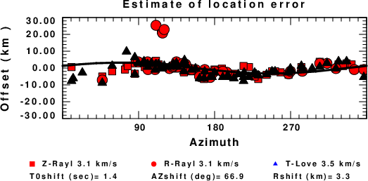
The derived shift in origin time and epicentral coordinates are given at the bottom of the figure.
Surface-Wave Focal Mechanism
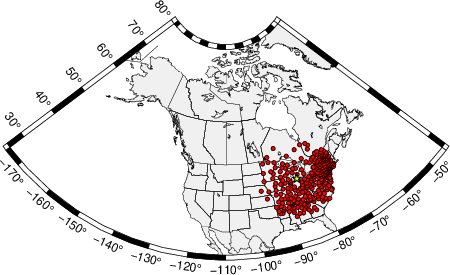
The following figure shows the stations used in the grid search for the best focal mechanism to fit the surface-wave spectral amplitudes of the Love and Rayleigh waves.
|
|
Location of broadband stations used to obtain focal mechanism from surface-wave spectral amplitudes
|
The surface-wave determined focal mechanism is shown here.
  NODAL PLANES


  STK=      24.56
  DIP=      85.02
 RAKE=     174.98

             OR

  STK=     114.99
  DIP=      85.00
 RAKE=       5.00


DEPTH = 7.0 km

Mw = 4.31
Best Fit 0.8634 - P-T axis plot gives solutions with FIT greater than FIT90
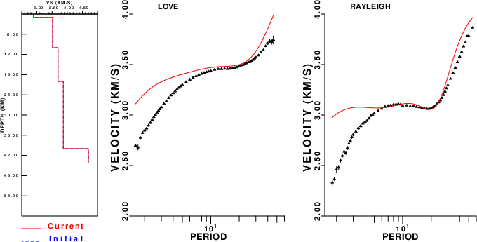
Surface-wave analysis
Surface wave analysis was performed using codes from
Computer Programs in Seismology, specifically the
multiple filter analysis program do_mft and the surface-wave
radiation pattern search program srfgrd96.
Data preparation
Digital data were collected, instrument response removed and traces converted
to Z, R an T components. Multiple filter analysis was applied to the Z and T traces to obtain the Rayleigh- and Love-wave spectral amplitudes, respectively.
These were input to the search program which examined all depths between 1 and 25 km
and all possible mechanisms.
|
|
Best mechanism fit as a function of depth. The preferred depth is given above. Lower hemisphere projection
|
|
|
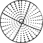
Pressure-tension axis trends. Since the surface-wave spectra search does not distinguish between P and T axes and since there is a 180 ambiguity in strike, all possible P and T axes are plotted. First motion data and waveforms will be used to select the preferred mechanism. The purpose of this plot is to provide an idea of the
possible range of solutions. The P and T-axes for all mechanisms with goodness of fit greater than 0.9 FITMAX (above) are plotted here.
|
|
|
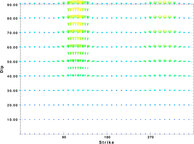
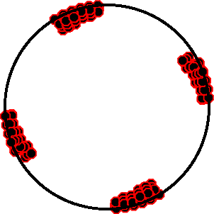
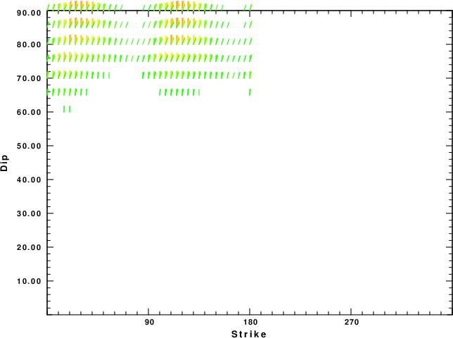
Focal mechanism sensitivity at the preferred depth. The red color indicates a very good fit to the Love and Rayleigh wave radiation patterns.
Each solution is plotted as a vector at a given value of strike and dip with the angle of the vector representing the rake angle, measured, with respect to the upward vertical (N) in the figure. Because of the symmetry of the spectral amplitude rediation patterns, only strikes from 0-180 degrees are sampled.
|
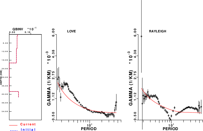
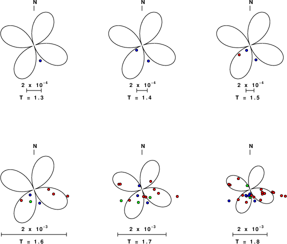
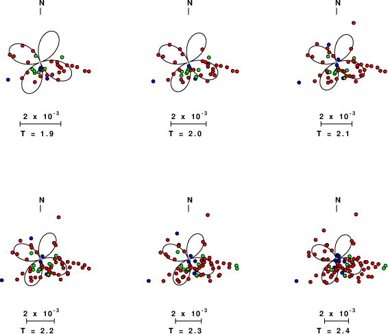
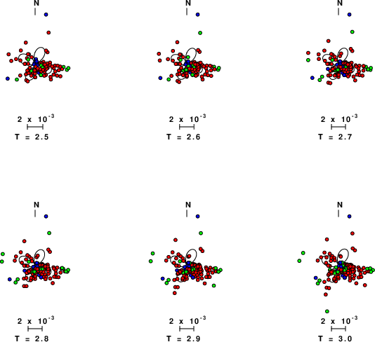
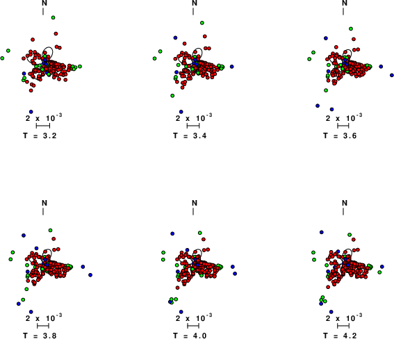
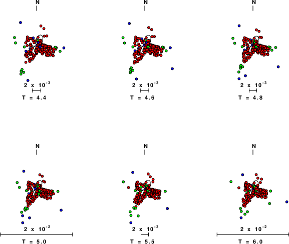
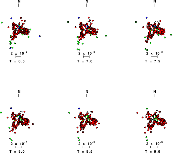
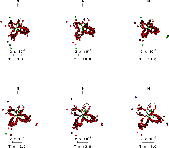
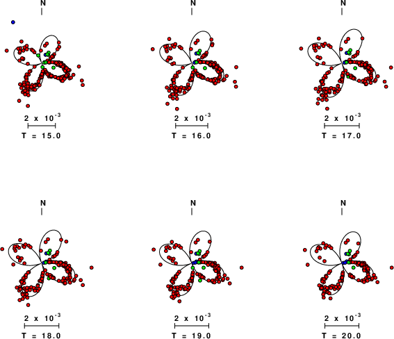
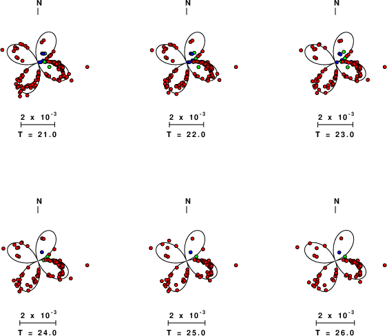
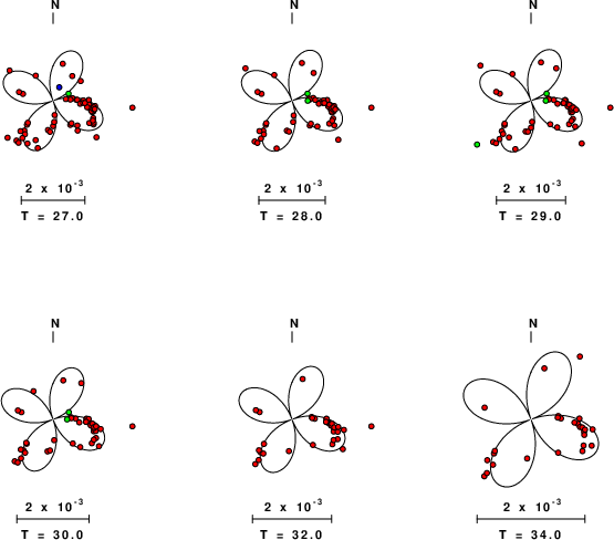
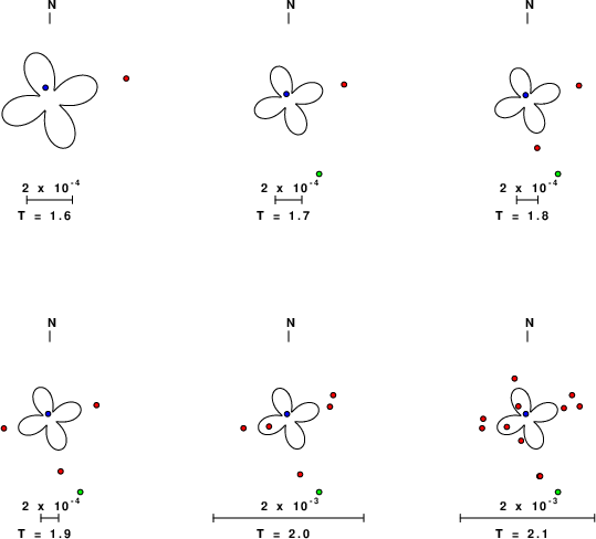
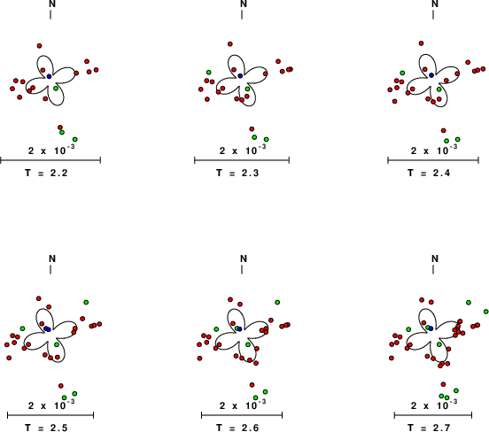
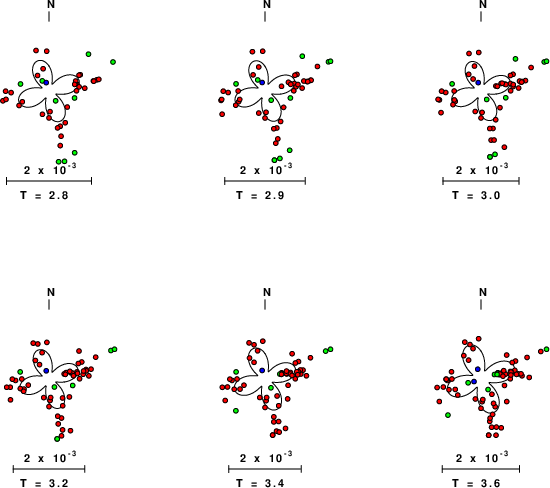
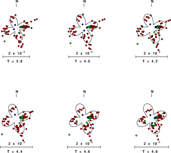
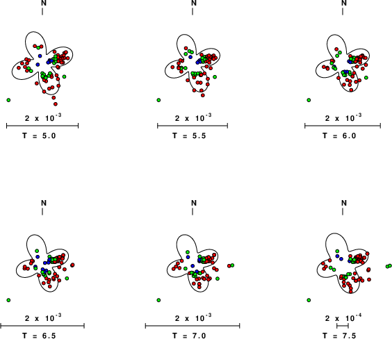
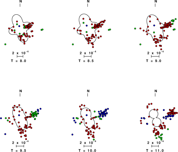
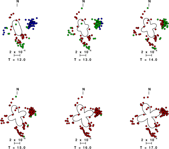
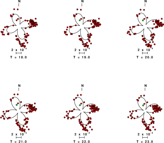
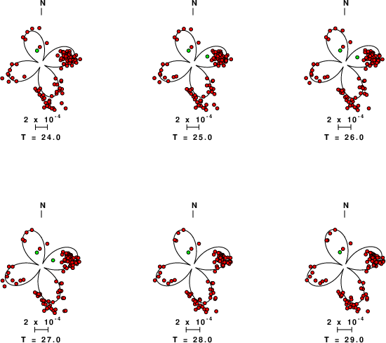
The next set of figures compares the observed and predicted surface wave radiation patterns as a function of period. The observed spectral amplitude have been corrected for anleastic attenuation by multiplication by a factor of eγr and corrected for surface wave geometrical spreading to a reference distance of 1000km. If the theoretical γ values are not perfect, then observations at large distance will plot as outliers.
Love-wave radiation patterns
Rayleigh-wave radiation patterns