Location
Location ANSS
The ANSS event ID is ak0152krol27 and the event page is at
https://earthquake.usgs.gov/earthquakes/eventpage/ak0152krol27/executive.
2015/02/25 09:38:48 63.194 -150.437 122.0 4.1 Alaska
Focal Mechanism
 USGS/SLU Moment Tensor Solution
 ENS  2015/02/25 09:38:48:0  63.19 -150.44 122.0 4.1 Alaska

 Stations used:
   AK.BPAW AK.BWN AK.CCB AK.HDA AK.KTH AK.MDM AK.PAX AK.RND
   AK.SAW AK.TRF AK.WRH AT.MENT AT.SVW2 AT.TTA IU.COLA TA.I23K
   TA.M24K

 Filtering commands used:
   cut o DIST/3.3 -50 o DIST/3.3 +50
   rtr
   taper w 0.1
   hp c 0.02 n 3
   lp c 0.05 n 3

 Best Fitting Double Couple
  Mo = 2.19e+22 dyne-cm
  Mw = 4.16
  Z  = 132 km
  Plane   Strike  Dip  Rake
   NP1      350    85    70
   NP2      247    21   166
  Principal Axes:
   Axis    Value   Plunge  Azimuth
    T   2.19e+22     46     239
    N   0.00e+00     20     352
    P  -2.19e+22     37      98

 Moment Tensor: (dyne-cm)
    Component   Value
       Mxx     2.44e+21
       Mxy     6.39e+21
       Mxz    -4.16e+21
       Myy    -6.01e+21
       Myz    -1.98e+22
       Mzz     3.57e+21


                     ----##########
                 --------##############
              --------####------------####
             ------#######---------------##
           -----###########-----------------#
          ----#############-------------------
         ----###############-------------------
        ---#################--------------------
        --##################--------------------
       ---###################--------------------
       --####################-----------   ------
       --####################----------- P ------
       -#########   ##########----------   ------
        ######### T ##########------------------
        -########   ##########------------------
         ######################----------------
          #####################---------------
           ####################--------------
             ##################------------
              #################-----------
                 ###############-------
                     ###########---


 Global CMT Convention Moment Tensor:
      R          T          P
  3.57e+21  -4.16e+21   1.98e+22
 -4.16e+21   2.44e+21  -6.39e+21
  1.98e+22  -6.39e+21  -6.01e+21


Details of the solution is found at

http://www.eas.slu.edu/eqc/eqc_mt/MECH.NA/20150225093848/index.html
|
Preferred Solution
The preferred solution from an analysis of the surface-wave spectral amplitude radiation pattern, waveform inversion or first motion observations is
      STK = 350
      DIP = 85
     RAKE = 70
       MW = 4.16
       HS = 132.0
The NDK file is 20150225093848.ndk
The waveform inversion is preferred.
Magnitudes
Given the availability of digital waveforms for determination of the moment tensor, this section documents the added processing leading to mLg, if appropriate to the region, and ML by application of the respective IASPEI formulae. As a research study, the linear distance term of the IASPEI formula
for ML is adjusted to remove a linear distance trend in residuals to give a regionally defined ML. The defined ML uses horizontal component recordings, but the same procedure is applied to the vertical components since there may be some interest in vertical component ground motions. Residual plots versus distance may indicate interesting features of ground motion scaling in some distance ranges. A residual plot of the regionalized magnitude is given as a function of distance and azimuth, since data sets may transcend different wave propagation provinces.
ML Magnitude
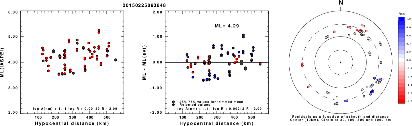
Left: ML computed using the IASPEI formula for Horizontal components. Center: ML residuals computed using a modified IASPEI formula that accounts for path specific attenuation; the values used for the trimmed mean are indicated. The ML relation used for each figure is given at the bottom of each plot.
Right: Residuals from new relation as a function of distance and azimuth.
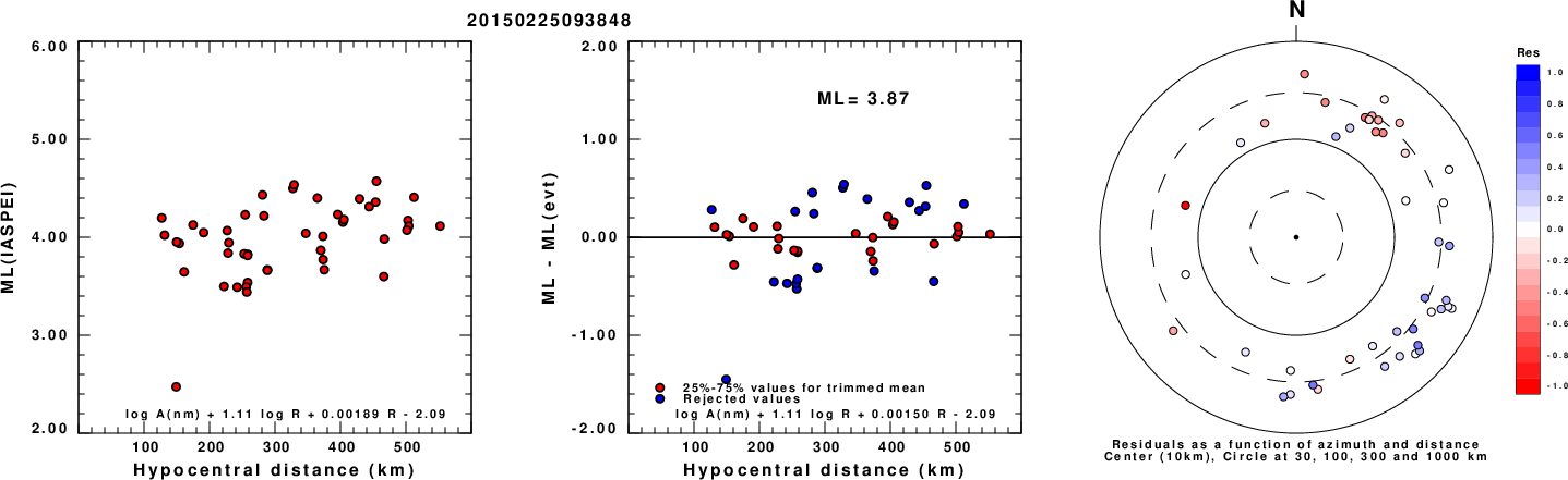
Left: ML computed using the IASPEI formula for Vertical components (research). Center: ML residuals computed using a modified IASPEI formula that accounts for path specific attenuation; the values used for the trimmed mean are indicated. The ML relation used for each figure is given at the bottom of each plot.
Right: Residuals from new relation as a function of distance and azimuth.
Context
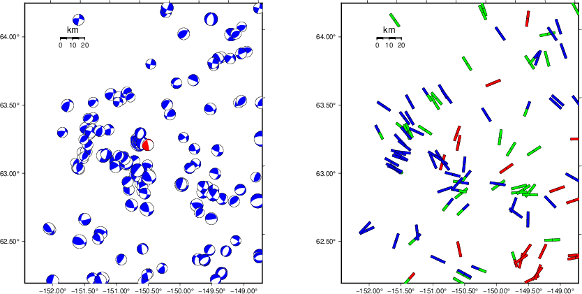
The left panel of the next figure presents the focal mechanism for this earthquake (red) in the context of other nearby events (blue) in the SLU Moment Tensor Catalog. The right panel shows the inferred direction of maximum compressive stress and the type of faulting (green is strike-slip, red is normal, blue is thrust; oblique is shown by a combination of colors). Thus context plot is useful for assessing the appropriateness of the moment tensor of this event.
Waveform Inversion using wvfgrd96
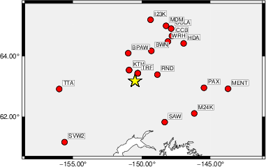
The focal mechanism was determined using broadband seismic waveforms. The location of the event (star) and the
stations used for (red) the waveform inversion are shown in the next figure.
|
|
Location of broadband stations used for waveform inversion
|
The program wvfgrd96 was used with good traces observed at short distance to determine the focal mechanism, depth and seismic moment. This technique requires a high quality signal and well determined velocity model for the Green's functions. To the extent that these are the quality data, this type of mechanism should be preferred over the radiation pattern technique which requires the separate step of defining the pressure and tension quadrants and the correct strike.
The observed and predicted traces are filtered using the following gsac commands:
cut o DIST/3.3 -50 o DIST/3.3 +50
rtr
taper w 0.1
hp c 0.02 n 3
lp c 0.05 n 3
The results of this grid search are as follow:
           DEPTH  STK   DIP  RAKE   MW    FIT
WVFGRD96    2.0    20    45   -75   3.43 0.1655
WVFGRD96    4.0    80    45   -20   3.40 0.1812
WVFGRD96    6.0    80    40   -15   3.46 0.1977
WVFGRD96    8.0    70    30   -30   3.57 0.2150
WVFGRD96   10.0    75    30   -20   3.60 0.2304
WVFGRD96   12.0    80    30   -15   3.62 0.2432
WVFGRD96   14.0    85    35    -5   3.62 0.2525
WVFGRD96   16.0    90    35     0   3.65 0.2585
WVFGRD96   18.0    90    35     0   3.67 0.2595
WVFGRD96   20.0    90    40     0   3.67 0.2568
WVFGRD96   22.0   100    40    20   3.68 0.2512
WVFGRD96   24.0   100    40    15   3.70 0.2446
WVFGRD96   26.0     5    80   -40   3.71 0.2493
WVFGRD96   28.0   195    75    50   3.74 0.2492
WVFGRD96   30.0     5    80   -45   3.76 0.2543
WVFGRD96   32.0     5    80   -40   3.77 0.2565
WVFGRD96   34.0     5    80   -40   3.78 0.2576
WVFGRD96   36.0     5    80   -35   3.79 0.2598
WVFGRD96   38.0     5    80   -30   3.81 0.2614
WVFGRD96   40.0     5    85   -35   3.87 0.2642
WVFGRD96   42.0     5    85   -30   3.87 0.2647
WVFGRD96   44.0    10    80   -40   3.94 0.2653
WVFGRD96   46.0     5    60   -15   3.88 0.2759
WVFGRD96   48.0     5    65   -10   3.88 0.2866
WVFGRD96   50.0     5    65   -10   3.90 0.2975
WVFGRD96   52.0     5    65    -5   3.90 0.3100
WVFGRD96   54.0     5    70    10   3.89 0.3238
WVFGRD96   56.0     5    70    15   3.90 0.3477
WVFGRD96   58.0     5    75    25   3.92 0.3782
WVFGRD96   60.0     5    75    25   3.94 0.4106
WVFGRD96   62.0     5    80    35   3.96 0.4464
WVFGRD96   64.0     5    80    40   3.98 0.4853
WVFGRD96   66.0    -5    90    40   3.99 0.5255
WVFGRD96   68.0     0    90    40   4.01 0.5658
WVFGRD96   70.0     0    90    40   4.03 0.6036
WVFGRD96   72.0     0    90    45   4.04 0.6396
WVFGRD96   74.0     0    90    50   4.06 0.6689
WVFGRD96   76.0     0    90    50   4.06 0.6881
WVFGRD96   78.0   175    90   -55   4.06 0.6979
WVFGRD96   80.0    -5    90    55   4.07 0.7066
WVFGRD96   82.0    -5    90    55   4.07 0.7140
WVFGRD96   84.0    -5    90    60   4.08 0.7231
WVFGRD96   86.0    -5    90    60   4.09 0.7302
WVFGRD96   88.0    -5    90    60   4.09 0.7385
WVFGRD96   90.0   175    90   -60   4.10 0.7446
WVFGRD96   92.0   175    90   -60   4.10 0.7512
WVFGRD96   94.0   355    90    60   4.10 0.7569
WVFGRD96   96.0   175    90   -60   4.11 0.7616
WVFGRD96   98.0   175    90   -60   4.11 0.7666
WVFGRD96  100.0   175    90   -65   4.12 0.7698
WVFGRD96  102.0   175    90   -65   4.12 0.7745
WVFGRD96  104.0   170    90   -65   4.12 0.7778
WVFGRD96  106.0   170    90   -65   4.12 0.7820
WVFGRD96  100.0   175    90   -65   4.12 0.7698
WVFGRD96  110.0   355    85    65   4.13 0.7885
WVFGRD96  112.0   170    90   -70   4.14 0.7915
WVFGRD96  114.0   170    90   -70   4.14 0.7942
WVFGRD96  116.0   170    90   -70   4.14 0.7970
WVFGRD96  118.0   170    90   -70   4.14 0.7986
WVFGRD96  120.0   170    90   -70   4.15 0.7997
WVFGRD96  122.0   170    90   -70   4.15 0.8000
WVFGRD96  124.0   170    90   -70   4.15 0.8019
WVFGRD96  126.0   350    85    70   4.15 0.8042
WVFGRD96  128.0   350    85    70   4.16 0.8060
WVFGRD96  130.0   170    90   -70   4.16 0.8023
WVFGRD96  132.0   350    85    70   4.16 0.8063
WVFGRD96  134.0   165    90   -75   4.17 0.8034
WVFGRD96  136.0   165    90   -75   4.17 0.8014
WVFGRD96  138.0   350    85    70   4.17 0.8054
WVFGRD96  140.0   350    85    70   4.17 0.8046
WVFGRD96  142.0   350    85    70   4.17 0.8025
WVFGRD96  144.0   350    85    70   4.18 0.8012
WVFGRD96  146.0   345    85    75   4.19 0.8006
WVFGRD96  148.0   345    85    75   4.19 0.7996
The best solution is
WVFGRD96 132.0 350 85 70 4.16 0.8063
The mechanism corresponding to the best fit is
|
|
Figure 1. Waveform inversion focal mechanism
|
The best fit as a function of depth is given in the following figure:
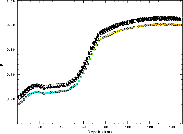
|
|
Figure 2. Depth sensitivity for waveform mechanism
|
The comparison of the observed and predicted waveforms is given in the next figure. The red traces are the observed and the blue are the predicted.
Each observed-predicted component is plotted to the same scale and peak amplitudes are indicated by the numbers to the left of each trace. A pair of numbers is given in black at the right of each predicted traces. The upper number it the time shift required for maximum correlation between the observed and predicted traces. This time shift is required because the synthetics are not computed at exactly the same distance as the observed, the velocity model used in the predictions may not be perfect and the epicentral parameters may be be off.
A positive time shift indicates that the prediction is too fast and should be delayed to match the observed trace (shift to the right in this figure). A negative value indicates that the prediction is too slow. The lower number gives the percentage of variance reduction to characterize the individual goodness of fit (100% indicates a perfect fit).
The bandpass filter used in the processing and for the display was
cut o DIST/3.3 -50 o DIST/3.3 +50
rtr
taper w 0.1
hp c 0.02 n 3
lp c 0.05 n 3
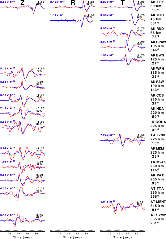
|
|
Figure 3. Waveform comparison for selected depth. Red: observed; Blue - predicted. The time shift with respect to the model prediction is indicated. The percent of fit is also indicated. The time scale is relative to the first trace sample.
|
|
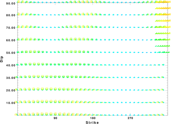
|
Focal mechanism sensitivity at the preferred depth. The red color indicates a very good fit to the waveforms.
Each solution is plotted as a vector at a given value of strike and dip with the angle of the vector representing the rake angle, measured, with respect to the upward vertical (N) in the figure.
|
A check on the assumed source location is possible by looking at the time shifts between the observed and predicted traces. The time shifts for waveform matching arise for several reasons:
- The origin time and epicentral distance are incorrect
- The velocity model used for the inversion is incorrect
- The velocity model used to define the P-arrival time is not the
same as the velocity model used for the waveform inversion
(assuming that the initial trace alignment is based on the
P arrival time)
Assuming only a mislocation, the time shifts are fit to a functional form:
Time_shift = A + B cos Azimuth + C Sin Azimuth
The time shifts for this inversion lead to the next figure:
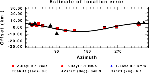
The derived shift in origin time and epicentral coordinates are given at the bottom of the figure.
Velocity Model
The WUS.model used for the waveform synthetic seismograms and for the surface wave eigenfunctions and dispersion is as follows
(The format is in the model96 format of Computer Programs in Seismology).
MODEL.01
Model after     8 iterations
ISOTROPIC
KGS
FLAT EARTH
1-D
CONSTANT VELOCITY
LINE08
LINE09
LINE10
LINE11
      H(KM)   VP(KM/S)   VS(KM/S) RHO(GM/CC)         QP         QS       ETAP       ETAS      FREFP      FREFS
     1.9000     3.4065     2.0089     2.2150  0.302E-02  0.679E-02   0.00       0.00       1.00       1.00
     6.1000     5.5445     3.2953     2.6089  0.349E-02  0.784E-02   0.00       0.00       1.00       1.00
    13.0000     6.2708     3.7396     2.7812  0.212E-02  0.476E-02   0.00       0.00       1.00       1.00
    19.0000     6.4075     3.7680     2.8223  0.111E-02  0.249E-02   0.00       0.00       1.00       1.00
     0.0000     7.9000     4.6200     3.2760  0.164E-10  0.370E-10   0.00       0.00       1.00       1.00
Last Changed Fri Apr 26 02:07:52 PM CDT 2024