Location
Location ANSS
The ANSS event ID is ak014fasfc4y and the event page is at
https://earthquake.usgs.gov/earthquakes/eventpage/ak014fasfc4y/executive.
2014/11/29 04:14:16 62.724 -150.485 97.1 5.1 Alaska
Focal Mechanism
 USGS/SLU Moment Tensor Solution
 ENS  2014/11/29 04:14:16:0  62.72 -150.49  97.1 5.1 Alaska

 Stations used:
   AK.BARN AK.BPAW AK.BRLK AK.BWN AK.CCB AK.CNP AK.DHY AK.DOT
   AK.GHO AK.GLB AK.GLI AK.HDA AK.HIN AK.HMT AK.ISLE AK.KLU
   AK.KNK AK.KTH AK.MCAR AK.MDM AK.MESA AK.PAX AK.PPLA AK.RAG
   AK.RIDG AK.RND AK.SAW AK.SCM AK.SKN AK.SSN AK.SWD AK.TABL
   AK.TGL AK.TRF AK.WRH AK.YAH AT.TTA IM.IL31 IU.COLA TA.I23K
   TA.K27K TA.M24K TA.N25K TA.O22K TA.POKR

 Filtering commands used:
   cut o DIST/3.3 -50 o DIST/3.3 +70
   rtr
   taper w 0.1
   hp c 0.02 n 3
   lp c 0.06 n 3

 Best Fitting Double Couple
  Mo = 3.35e+23 dyne-cm
  Mw = 4.95
  Z  = 106 km
  Plane   Strike  Dip  Rake
   NP1      352    66   141
   NP2      100    55    30
  Principal Axes:
   Axis    Value   Plunge  Azimuth
    T   3.35e+23     44     312
    N   0.00e+00     45     145
    P  -3.35e+23      7      48

 Moment Tensor: (dyne-cm)
    Component   Value
       Mxx    -7.14e+22
       Mxy    -2.50e+23
       Mxz     8.53e+22
       Myy    -8.60e+22
       Myz    -1.54e+23
       Mzz     1.57e+23


                     #####---------
                 ###########-----------
              ###############-------------
             #################------------
           ####################----------- P
          ########   ###########----------   -
         ######### T ###########---------------
        ##########   ############---------------
        #########################---------------
       -##########################---------------
       --#########################---------------
       ----#######################---------------
       ------#####################---------------
        -------####################------------#
        -----------################---------####
         ----------------##########-----#######
          ------------------------############
           -----------------------###########
             ---------------------#########
              -------------------#########
                 ----------------######
                     -----------###


 Global CMT Convention Moment Tensor:
      R          T          P
  1.57e+23   8.53e+22   1.54e+23
  8.53e+22  -7.14e+22   2.50e+23
  1.54e+23   2.50e+23  -8.60e+22


Details of the solution is found at

http://www.eas.slu.edu/eqc/eqc_mt/MECH.NA/20141129041416/index.html
|
Preferred Solution
The preferred solution from an analysis of the surface-wave spectral amplitude radiation pattern, waveform inversion or first motion observations is
      STK = 100
      DIP = 55
     RAKE = 30
       MW = 4.95
       HS = 106.0
The NDK file is 20141129041416.ndk
The waveform inversion is preferred.
Moment Tensor Comparison
The following compares this source inversion to those provided by others. The purpose is to look for major differences and also to note slight differences that might be inherent to the processing procedure. For completeness the USGS/SLU solution is repeated from above.
| SLU |
USGSMT |
 USGS/SLU Moment Tensor Solution
 ENS  2014/11/29 04:14:16:0  62.72 -150.49  97.1 5.1 Alaska

 Stations used:
   AK.BARN AK.BPAW AK.BRLK AK.BWN AK.CCB AK.CNP AK.DHY AK.DOT
   AK.GHO AK.GLB AK.GLI AK.HDA AK.HIN AK.HMT AK.ISLE AK.KLU
   AK.KNK AK.KTH AK.MCAR AK.MDM AK.MESA AK.PAX AK.PPLA AK.RAG
   AK.RIDG AK.RND AK.SAW AK.SCM AK.SKN AK.SSN AK.SWD AK.TABL
   AK.TGL AK.TRF AK.WRH AK.YAH AT.TTA IM.IL31 IU.COLA TA.I23K
   TA.K27K TA.M24K TA.N25K TA.O22K TA.POKR

 Filtering commands used:
   cut o DIST/3.3 -50 o DIST/3.3 +70
   rtr
   taper w 0.1
   hp c 0.02 n 3
   lp c 0.06 n 3

 Best Fitting Double Couple
  Mo = 3.35e+23 dyne-cm
  Mw = 4.95
  Z  = 106 km
  Plane   Strike  Dip  Rake
   NP1      352    66   141
   NP2      100    55    30
  Principal Axes:
   Axis    Value   Plunge  Azimuth
    T   3.35e+23     44     312
    N   0.00e+00     45     145
    P  -3.35e+23      7      48

 Moment Tensor: (dyne-cm)
    Component   Value
       Mxx    -7.14e+22
       Mxy    -2.50e+23
       Mxz     8.53e+22
       Myy    -8.60e+22
       Myz    -1.54e+23
       Mzz     1.57e+23


                     #####---------
                 ###########-----------
              ###############-------------
             #################------------
           ####################----------- P
          ########   ###########----------   -
         ######### T ###########---------------
        ##########   ############---------------
        #########################---------------
       -##########################---------------
       --#########################---------------
       ----#######################---------------
       ------#####################---------------
        -------####################------------#
        -----------################---------####
         ----------------##########-----#######
          ------------------------############
           -----------------------###########
             ---------------------#########
              -------------------#########
                 ----------------######
                     -----------###


 Global CMT Convention Moment Tensor:
      R          T          P
  1.57e+23   8.53e+22   1.54e+23
  8.53e+22  -7.14e+22   2.50e+23
  1.54e+23   2.50e+23  -8.60e+22


Details of the solution is found at

http://www.eas.slu.edu/eqc/eqc_mt/MECH.NA/20141129041416/index.html
|
Moment 3.34e+16 N-m
Magnitude 4.9
Percent DC 81%
Depth 99.0 km
Updated 2014-11-29 05:28:59 UTC
Author us
Catalog us
Contributor Code us_b000t12u_mwr
Principal Axes

Axis	Value	Plunge	Azimuth
T	3.492	47	310
N	-0.320	42	146
P	-3.173	8	48

|
Magnitudes
Given the availability of digital waveforms for determination of the moment tensor, this section documents the added processing leading to mLg, if appropriate to the region, and ML by application of the respective IASPEI formulae. As a research study, the linear distance term of the IASPEI formula
for ML is adjusted to remove a linear distance trend in residuals to give a regionally defined ML. The defined ML uses horizontal component recordings, but the same procedure is applied to the vertical components since there may be some interest in vertical component ground motions. Residual plots versus distance may indicate interesting features of ground motion scaling in some distance ranges. A residual plot of the regionalized magnitude is given as a function of distance and azimuth, since data sets may transcend different wave propagation provinces.
ML Magnitude
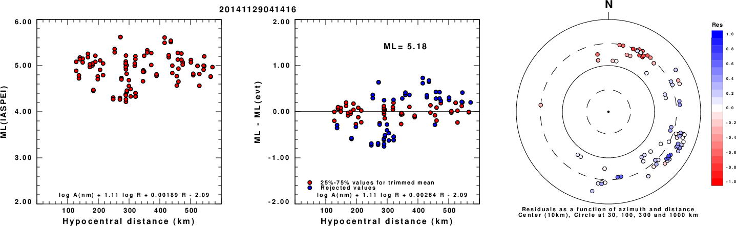
Left: ML computed using the IASPEI formula for Horizontal components. Center: ML residuals computed using a modified IASPEI formula that accounts for path specific attenuation; the values used for the trimmed mean are indicated. The ML relation used for each figure is given at the bottom of each plot.
Right: Residuals from new relation as a function of distance and azimuth.
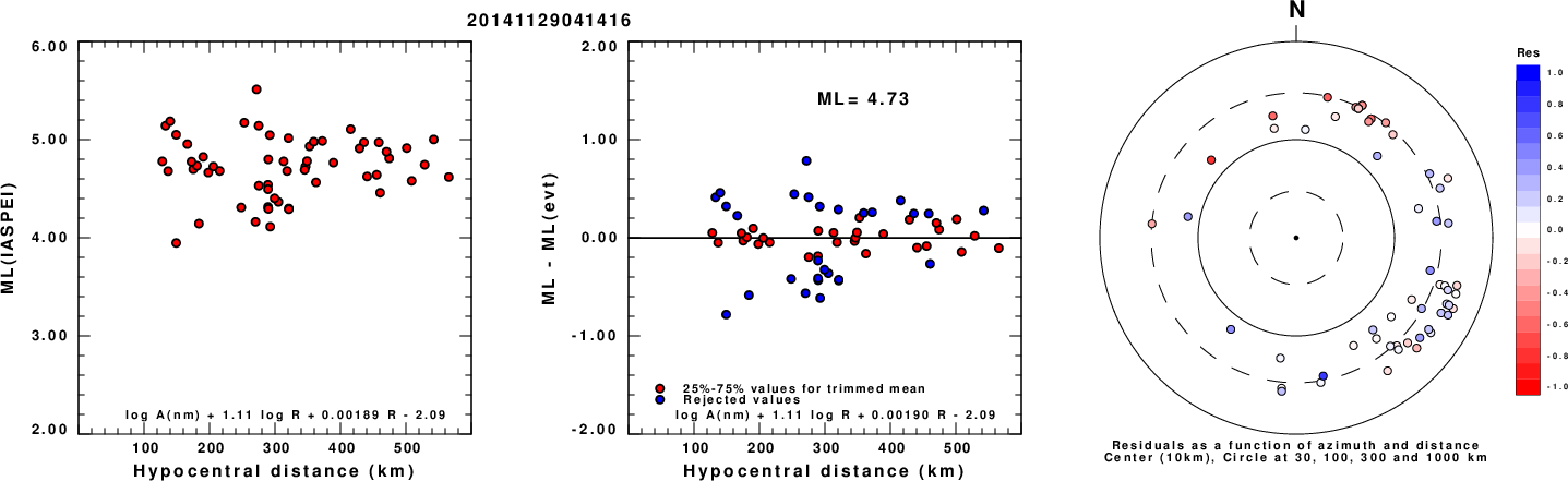
Left: ML computed using the IASPEI formula for Vertical components (research). Center: ML residuals computed using a modified IASPEI formula that accounts for path specific attenuation; the values used for the trimmed mean are indicated. The ML relation used for each figure is given at the bottom of each plot.
Right: Residuals from new relation as a function of distance and azimuth.
Context
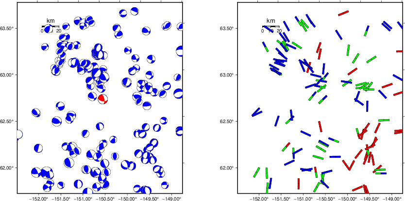
The left panel of the next figure presents the focal mechanism for this earthquake (red) in the context of other nearby events (blue) in the SLU Moment Tensor Catalog. The right panel shows the inferred direction of maximum compressive stress and the type of faulting (green is strike-slip, red is normal, blue is thrust; oblique is shown by a combination of colors). Thus context plot is useful for assessing the appropriateness of the moment tensor of this event.
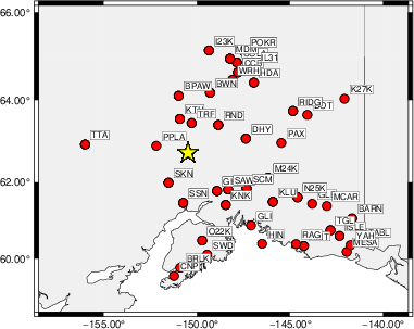
Waveform Inversion using wvfgrd96
The focal mechanism was determined using broadband seismic waveforms. The location of the event (star) and the
stations used for (red) the waveform inversion are shown in the next figure.
|
|
Location of broadband stations used for waveform inversion
|
The program wvfgrd96 was used with good traces observed at short distance to determine the focal mechanism, depth and seismic moment. This technique requires a high quality signal and well determined velocity model for the Green's functions. To the extent that these are the quality data, this type of mechanism should be preferred over the radiation pattern technique which requires the separate step of defining the pressure and tension quadrants and the correct strike.
The observed and predicted traces are filtered using the following gsac commands:
cut o DIST/3.3 -50 o DIST/3.3 +70
rtr
taper w 0.1
hp c 0.02 n 3
lp c 0.06 n 3
The results of this grid search are as follow:
           DEPTH  STK   DIP  RAKE   MW    FIT
WVFGRD96    2.0   145    45   -95   4.16 0.2667
WVFGRD96    4.0   170    45   -55   4.21 0.2358
WVFGRD96    6.0     5    45   -20   4.20 0.2498
WVFGRD96    8.0     5    45   -20   4.26 0.2704
WVFGRD96   10.0    10    50   -10   4.27 0.2815
WVFGRD96   12.0    10    50    -5   4.28 0.2905
WVFGRD96   14.0    15    50    10   4.30 0.2974
WVFGRD96   16.0    15    55    10   4.32 0.3021
WVFGRD96   18.0   300    60    45   4.34 0.3066
WVFGRD96   20.0   300    60    45   4.35 0.3127
WVFGRD96   22.0   295    60    40   4.38 0.3169
WVFGRD96   24.0   110    85    35   4.40 0.3209
WVFGRD96   26.0   110    80    35   4.42 0.3248
WVFGRD96   28.0   110    80    35   4.43 0.3281
WVFGRD96   30.0   105    85    30   4.46 0.3302
WVFGRD96   32.0   105    90    30   4.48 0.3332
WVFGRD96   34.0   105    90    30   4.49 0.3351
WVFGRD96   36.0   105    90    30   4.51 0.3354
WVFGRD96   38.0   285    85   -25   4.55 0.3388
WVFGRD96   40.0   285    90   -35   4.62 0.3407
WVFGRD96   42.0   285    85   -35   4.63 0.3415
WVFGRD96   44.0   285    90   -30   4.65 0.3418
WVFGRD96   46.0   105    90    30   4.66 0.3421
WVFGRD96   48.0   105    80    30   4.68 0.3440
WVFGRD96   50.0   100    65   -15   4.71 0.3505
WVFGRD96   52.0   100    65   -15   4.72 0.3585
WVFGRD96   54.0   100    65   -15   4.74 0.3660
WVFGRD96   56.0   100    45    25   4.77 0.3881
WVFGRD96   58.0   100    45    25   4.79 0.4074
WVFGRD96   60.0   100    50    30   4.80 0.4294
WVFGRD96   62.0   100    50    30   4.82 0.4544
WVFGRD96   64.0   100    50    30   4.83 0.4812
WVFGRD96   66.0   100    50    30   4.85 0.5080
WVFGRD96   68.0   105    45    35   4.86 0.5341
WVFGRD96   70.0   100    50    30   4.87 0.5591
WVFGRD96   72.0   100    50    30   4.88 0.5853
WVFGRD96   74.0   100    50    30   4.89 0.6113
WVFGRD96   76.0   105    50    35   4.90 0.6354
WVFGRD96   78.0   105    50    35   4.91 0.6589
WVFGRD96   80.0   105    50    35   4.91 0.6797
WVFGRD96   82.0   105    50    35   4.92 0.6986
WVFGRD96   84.0   105    50    35   4.93 0.7149
WVFGRD96   86.0   105    50    35   4.93 0.7288
WVFGRD96   88.0   105    50    35   4.93 0.7408
WVFGRD96   90.0   105    50    35   4.93 0.7501
WVFGRD96   92.0   105    50    35   4.94 0.7577
WVFGRD96   94.0   105    50    35   4.94 0.7636
WVFGRD96   96.0   105    50    35   4.94 0.7676
WVFGRD96   98.0   105    50    35   4.94 0.7705
WVFGRD96  100.0   105    50    35   4.94 0.7720
WVFGRD96  102.0   105    50    35   4.94 0.7726
WVFGRD96  104.0   100    55    30   4.95 0.7728
WVFGRD96  106.0   100    55    30   4.95 0.7733
WVFGRD96  108.0   100    55    30   4.95 0.7731
WVFGRD96  110.0   100    55    30   4.95 0.7719
WVFGRD96  112.0   100    55    30   4.95 0.7698
WVFGRD96  114.0   100    55    30   4.95 0.7672
WVFGRD96  116.0   100    55    30   4.95 0.7642
WVFGRD96  118.0   100    55    30   4.95 0.7611
The best solution is
WVFGRD96 106.0 100 55 30 4.95 0.7733
The mechanism corresponding to the best fit is
|
|
Figure 1. Waveform inversion focal mechanism
|
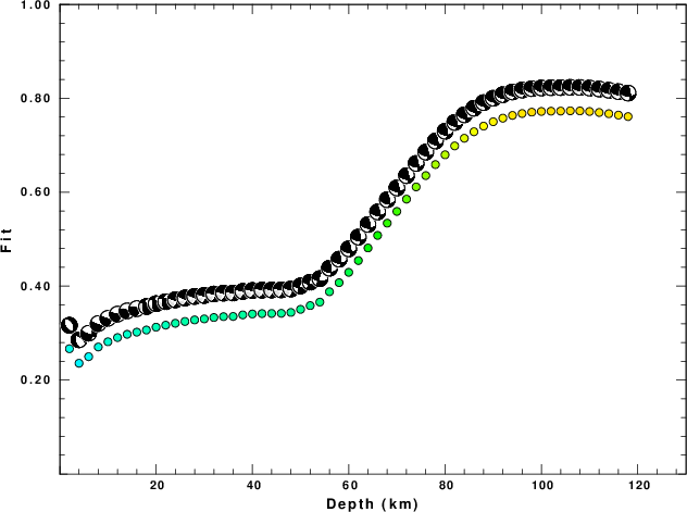
The best fit as a function of depth is given in the following figure:
|
|
Figure 2. Depth sensitivity for waveform mechanism
|
The comparison of the observed and predicted waveforms is given in the next figure. The red traces are the observed and the blue are the predicted.
Each observed-predicted component is plotted to the same scale and peak amplitudes are indicated by the numbers to the left of each trace. A pair of numbers is given in black at the right of each predicted traces. The upper number it the time shift required for maximum correlation between the observed and predicted traces. This time shift is required because the synthetics are not computed at exactly the same distance as the observed, the velocity model used in the predictions may not be perfect and the epicentral parameters may be be off.
A positive time shift indicates that the prediction is too fast and should be delayed to match the observed trace (shift to the right in this figure). A negative value indicates that the prediction is too slow. The lower number gives the percentage of variance reduction to characterize the individual goodness of fit (100% indicates a perfect fit).
The bandpass filter used in the processing and for the display was
cut o DIST/3.3 -50 o DIST/3.3 +70
rtr
taper w 0.1
hp c 0.02 n 3
lp c 0.06 n 3
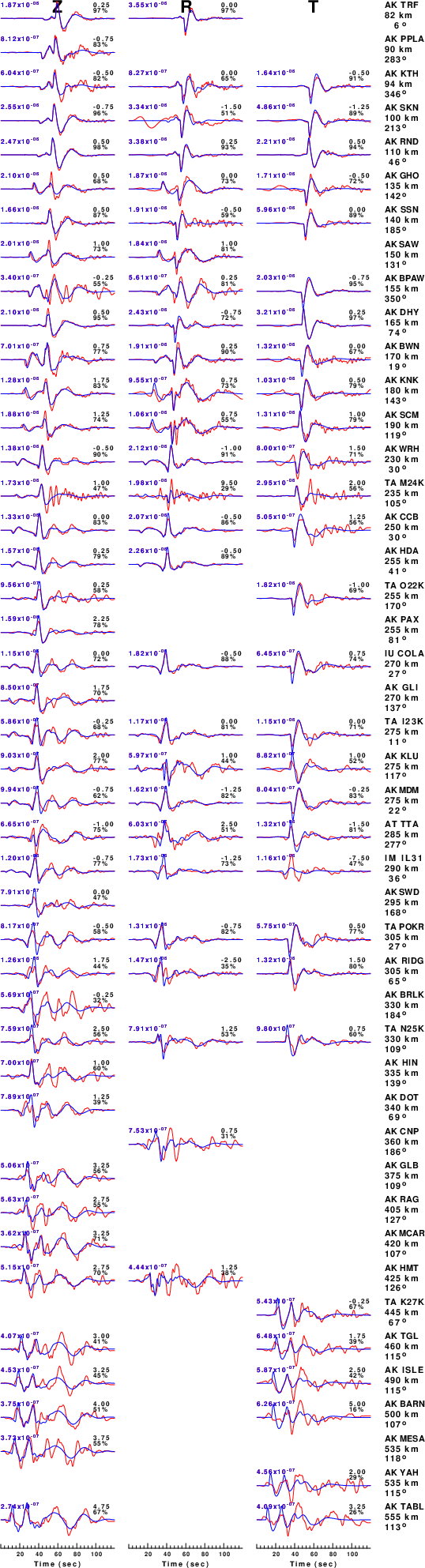
|
|
Figure 3. Waveform comparison for selected depth. Red: observed; Blue - predicted. The time shift with respect to the model prediction is indicated. The percent of fit is also indicated. The time scale is relative to the first trace sample.
|
|
|
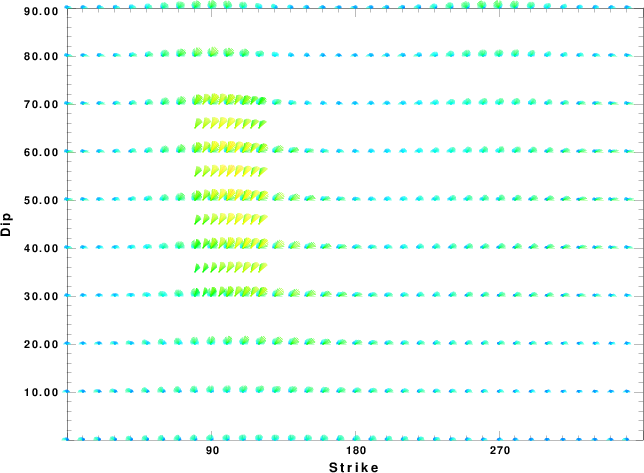
Focal mechanism sensitivity at the preferred depth. The red color indicates a very good fit to the waveforms.
Each solution is plotted as a vector at a given value of strike and dip with the angle of the vector representing the rake angle, measured, with respect to the upward vertical (N) in the figure.
|
A check on the assumed source location is possible by looking at the time shifts between the observed and predicted traces. The time shifts for waveform matching arise for several reasons:
- The origin time and epicentral distance are incorrect
- The velocity model used for the inversion is incorrect
- The velocity model used to define the P-arrival time is not the
same as the velocity model used for the waveform inversion
(assuming that the initial trace alignment is based on the
P arrival time)
Assuming only a mislocation, the time shifts are fit to a functional form:
Time_shift = A + B cos Azimuth + C Sin Azimuth
The time shifts for this inversion lead to the next figure:
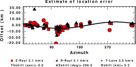
The derived shift in origin time and epicentral coordinates are given at the bottom of the figure.
Velocity Model
The WUS.model used for the waveform synthetic seismograms and for the surface wave eigenfunctions and dispersion is as follows
(The format is in the model96 format of Computer Programs in Seismology).
MODEL.01
Model after     8 iterations
ISOTROPIC
KGS
FLAT EARTH
1-D
CONSTANT VELOCITY
LINE08
LINE09
LINE10
LINE11
      H(KM)   VP(KM/S)   VS(KM/S) RHO(GM/CC)         QP         QS       ETAP       ETAS      FREFP      FREFS
     1.9000     3.4065     2.0089     2.2150  0.302E-02  0.679E-02   0.00       0.00       1.00       1.00
     6.1000     5.5445     3.2953     2.6089  0.349E-02  0.784E-02   0.00       0.00       1.00       1.00
    13.0000     6.2708     3.7396     2.7812  0.212E-02  0.476E-02   0.00       0.00       1.00       1.00
    19.0000     6.4075     3.7680     2.8223  0.111E-02  0.249E-02   0.00       0.00       1.00       1.00
     0.0000     7.9000     4.6200     3.2760  0.164E-10  0.370E-10   0.00       0.00       1.00       1.00
Last Changed Sat Apr 27 03:41:23 AM CDT 2024