Location
Location ANSS
The ANSS event ID is ak014cn5hnbt and the event page is at
https://earthquake.usgs.gov/earthquakes/eventpage/ak014cn5hnbt/executive.
2014/10/02 21:33:15 63.055 -150.775 123.6 4.3 Alaska
Focal Mechanism
 USGS/SLU Moment Tensor Solution
 ENS  2014/10/02 21:33:15:0  63.06 -150.77 123.6 4.3 Alaska

 Stations used:
   AK.BPAW AK.BWN AK.CRQ AK.DHY AK.DOT AK.EYAK AK.FID AK.GHO
   AK.GLB AK.GLI AK.HDA AK.HIN AK.KLU AK.KNK AK.KTH AK.MCAR
   AK.MDM AK.PAX AK.PPLA AK.RIDG AK.RND AK.SAW AK.SCM AK.SKN
   AK.SSN AK.SWD AK.TRF AK.WRH IM.IL31 IU.COLA TA.M24K

 Filtering commands used:
   cut o DIST/3.3 -50 o DIST/3.3 +60
   rtr
   taper w 0.1
   hp c 0.02 n 3
   lp c 0.06 n 3

 Best Fitting Double Couple
  Mo = 3.55e+22 dyne-cm
  Mw = 4.30
  Z  = 122 km
  Plane   Strike  Dip  Rake
   NP1       50    70    85
   NP2      244    21   103
  Principal Axes:
   Axis    Value   Plunge  Azimuth
    T   3.55e+22     65     312
    N   0.00e+00      5      52
    P  -3.55e+22     25     144

 Moment Tensor: (dyne-cm)
    Component   Value
       Mxx    -1.62e+22
       Mxy     1.07e+22
       Mxz     2.01e+22
       Myy    -6.53e+21
       Myz    -1.82e+22
       Mzz     2.27e+22


                     --------------
                 ----------------------
              --------################----
             ------#######################-
           -----#############################
          ----#############################---
         ----#############################-----
        ---###########   ################-------
        --############ T ##############---------
       ---############   #############-----------
       --###########################-------------
       --##########################--------------
       --########################----------------
        -#####################------------------
        -###################--------------------
         ################----------------------
          ############--------------   -------
           #######------------------ P ------
             -----------------------   ----
              ----------------------------
                 ----------------------
                     --------------


 Global CMT Convention Moment Tensor:
      R          T          P
  2.27e+22   2.01e+22   1.82e+22
  2.01e+22  -1.62e+22  -1.07e+22
  1.82e+22  -1.07e+22  -6.53e+21


Details of the solution is found at

http://www.eas.slu.edu/eqc/eqc_mt/MECH.NA/20141002213315/index.html
|
Preferred Solution
The preferred solution from an analysis of the surface-wave spectral amplitude radiation pattern, waveform inversion or first motion observations is
      STK = 50
      DIP = 70
     RAKE = 85
       MW = 4.30
       HS = 122.0
The NDK file is 20141002213315.ndk
The waveform inversion is preferred.
Magnitudes
Given the availability of digital waveforms for determination of the moment tensor, this section documents the added processing leading to mLg, if appropriate to the region, and ML by application of the respective IASPEI formulae. As a research study, the linear distance term of the IASPEI formula
for ML is adjusted to remove a linear distance trend in residuals to give a regionally defined ML. The defined ML uses horizontal component recordings, but the same procedure is applied to the vertical components since there may be some interest in vertical component ground motions. Residual plots versus distance may indicate interesting features of ground motion scaling in some distance ranges. A residual plot of the regionalized magnitude is given as a function of distance and azimuth, since data sets may transcend different wave propagation provinces.
ML Magnitude
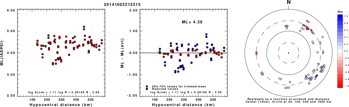
Left: ML computed using the IASPEI formula for Horizontal components. Center: ML residuals computed using a modified IASPEI formula that accounts for path specific attenuation; the values used for the trimmed mean are indicated. The ML relation used for each figure is given at the bottom of each plot.
Right: Residuals from new relation as a function of distance and azimuth.
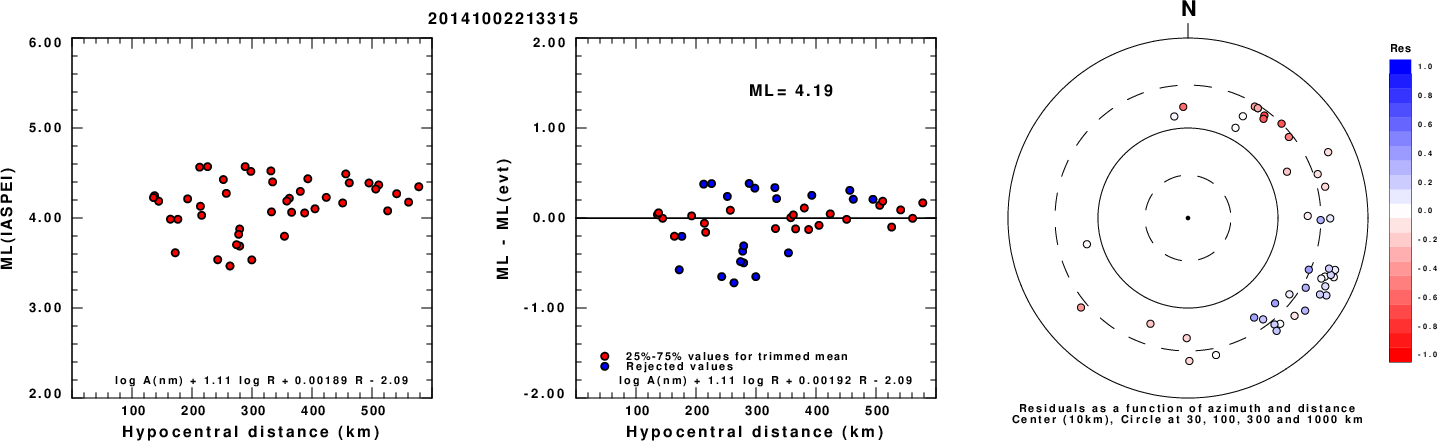
Left: ML computed using the IASPEI formula for Vertical components (research). Center: ML residuals computed using a modified IASPEI formula that accounts for path specific attenuation; the values used for the trimmed mean are indicated. The ML relation used for each figure is given at the bottom of each plot.
Right: Residuals from new relation as a function of distance and azimuth.
Context
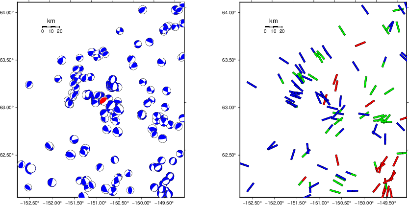
The left panel of the next figure presents the focal mechanism for this earthquake (red) in the context of other nearby events (blue) in the SLU Moment Tensor Catalog. The right panel shows the inferred direction of maximum compressive stress and the type of faulting (green is strike-slip, red is normal, blue is thrust; oblique is shown by a combination of colors). Thus context plot is useful for assessing the appropriateness of the moment tensor of this event.
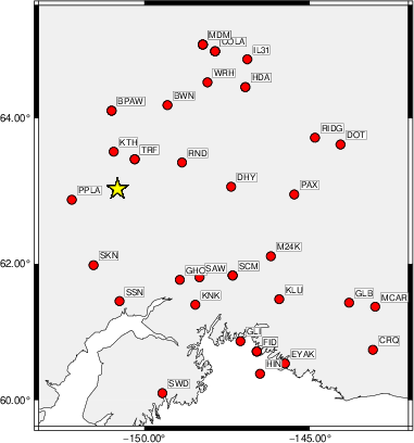
Waveform Inversion using wvfgrd96
The focal mechanism was determined using broadband seismic waveforms. The location of the event (star) and the
stations used for (red) the waveform inversion are shown in the next figure.
|
|
Location of broadband stations used for waveform inversion
|
The program wvfgrd96 was used with good traces observed at short distance to determine the focal mechanism, depth and seismic moment. This technique requires a high quality signal and well determined velocity model for the Green's functions. To the extent that these are the quality data, this type of mechanism should be preferred over the radiation pattern technique which requires the separate step of defining the pressure and tension quadrants and the correct strike.
The observed and predicted traces are filtered using the following gsac commands:
cut o DIST/3.3 -50 o DIST/3.3 +60
rtr
taper w 0.1
hp c 0.02 n 3
lp c 0.06 n 3
The results of this grid search are as follow:
           DEPTH  STK   DIP  RAKE   MW    FIT
WVFGRD96    2.0   240    50   -90   3.48 0.1780
WVFGRD96    4.0    70    35   -75   3.58 0.1646
WVFGRD96    6.0    60    30   -80   3.58 0.1381
WVFGRD96    8.0    60    30   -80   3.66 0.1560
WVFGRD96   10.0    70    30   -70   3.63 0.1468
WVFGRD96   12.0    30    30    75   3.64 0.1634
WVFGRD96   14.0    30    40    75   3.67 0.1840
WVFGRD96   16.0    30    40    70   3.67 0.2019
WVFGRD96   18.0    30    45    70   3.69 0.2154
WVFGRD96   20.0    30    45    70   3.70 0.2257
WVFGRD96   22.0    30    45    70   3.71 0.2317
WVFGRD96   24.0    30    45    70   3.72 0.2352
WVFGRD96   26.0    30    45    70   3.73 0.2365
WVFGRD96   28.0    25    45    65   3.74 0.2358
WVFGRD96   30.0    25    45    65   3.75 0.2337
WVFGRD96   32.0    25    45    65   3.76 0.2302
WVFGRD96   34.0    30    40    70   3.77 0.2255
WVFGRD96   36.0    10    40    65   3.79 0.2199
WVFGRD96   38.0    20    55    75   3.82 0.2155
WVFGRD96   40.0    20    60    80   3.97 0.2142
WVFGRD96   42.0    25    60    85   3.99 0.2151
WVFGRD96   44.0    25    60    80   3.99 0.2159
WVFGRD96   46.0    30    55    80   4.00 0.2169
WVFGRD96   48.0    25    60    75   4.00 0.2201
WVFGRD96   50.0    25    60    70   4.01 0.2241
WVFGRD96   52.0    10    60    25   4.00 0.2331
WVFGRD96   54.0    15    60    30   4.01 0.2457
WVFGRD96   56.0    15    60    25   4.04 0.2597
WVFGRD96   58.0    15    60    25   4.06 0.2753
WVFGRD96   60.0    20    60    25   4.07 0.2929
WVFGRD96   62.0    35    75    80   4.10 0.3248
WVFGRD96   64.0    35    75    80   4.12 0.3609
WVFGRD96   66.0    40    70    80   4.14 0.3976
WVFGRD96   68.0    40    75    75   4.15 0.4351
WVFGRD96   70.0    45    70    80   4.17 0.4686
WVFGRD96   72.0    45    70    80   4.18 0.4937
WVFGRD96   74.0    45    70    80   4.19 0.5106
WVFGRD96   76.0    45    70    85   4.20 0.5269
WVFGRD96   78.0   240    20   100   4.21 0.5416
WVFGRD96   80.0    45    70    85   4.22 0.5575
WVFGRD96   82.0   240    20   100   4.22 0.5720
WVFGRD96   84.0    50    70    85   4.23 0.5836
WVFGRD96   86.0    50    70    85   4.23 0.5966
WVFGRD96   88.0    50    70    90   4.24 0.6071
WVFGRD96   90.0    50    70    90   4.25 0.6170
WVFGRD96   92.0    50    70    90   4.25 0.6258
WVFGRD96   94.0    50    65    80   4.25 0.6327
WVFGRD96   96.0    50    65    80   4.25 0.6423
WVFGRD96   98.0    50    65    80   4.26 0.6498
WVFGRD96  100.0    50    65    80   4.26 0.6567
WVFGRD96  102.0    50    65    80   4.27 0.6623
WVFGRD96  104.0    50    65    80   4.27 0.6673
WVFGRD96  106.0    50    70    85   4.28 0.6717
WVFGRD96  108.0    50    70    85   4.28 0.6754
WVFGRD96  110.0    50    70    85   4.28 0.6788
WVFGRD96  112.0    50    70    85   4.29 0.6814
WVFGRD96  114.0    50    70    85   4.29 0.6838
WVFGRD96  116.0    50    70    85   4.29 0.6848
WVFGRD96  118.0    50    70    85   4.29 0.6864
WVFGRD96  120.0    50    70    85   4.30 0.6864
WVFGRD96  122.0    50    70    85   4.30 0.6867
WVFGRD96  124.0   235    20    95   4.30 0.6856
WVFGRD96  126.0   235    20    95   4.31 0.6847
WVFGRD96  128.0    50    70    85   4.30 0.6842
WVFGRD96  130.0    50    70    85   4.31 0.6822
WVFGRD96  132.0    50    70    85   4.31 0.6816
WVFGRD96  134.0    50    70    85   4.31 0.6793
WVFGRD96  136.0    50    70    85   4.31 0.6775
WVFGRD96  138.0    55    70    90   4.32 0.6751
WVFGRD96  140.0   240    20    95   4.32 0.6731
WVFGRD96  142.0   240    20    95   4.32 0.6709
WVFGRD96  144.0    55    70    90   4.33 0.6673
WVFGRD96  146.0    55    70    90   4.33 0.6648
WVFGRD96  148.0    55    70    90   4.33 0.6619
The best solution is
WVFGRD96 122.0 50 70 85 4.30 0.6867
The mechanism corresponding to the best fit is
|
|
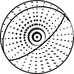
Figure 1. Waveform inversion focal mechanism
|
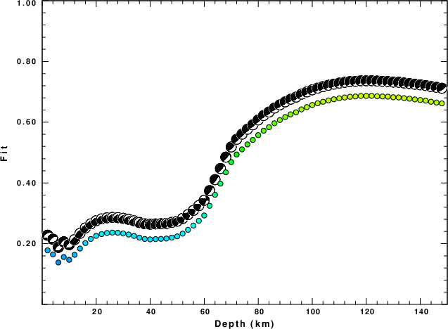
The best fit as a function of depth is given in the following figure:
|
|
Figure 2. Depth sensitivity for waveform mechanism
|
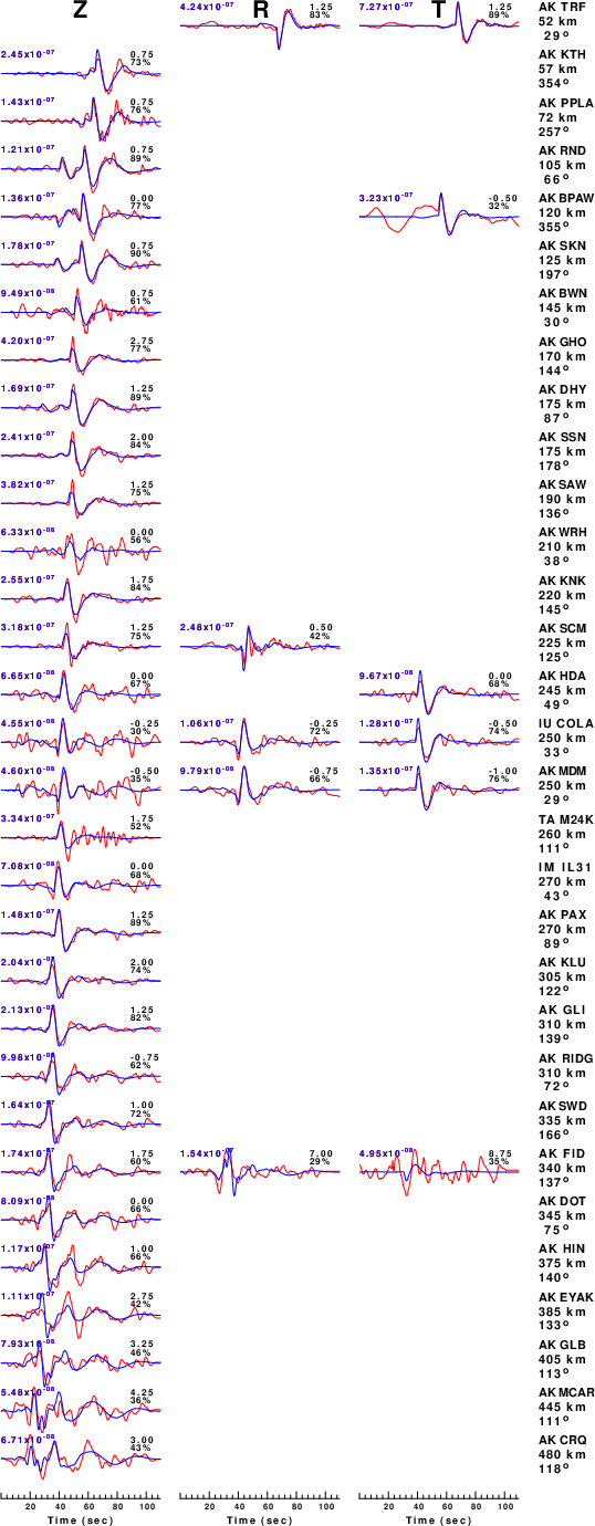
The comparison of the observed and predicted waveforms is given in the next figure. The red traces are the observed and the blue are the predicted.
Each observed-predicted component is plotted to the same scale and peak amplitudes are indicated by the numbers to the left of each trace. A pair of numbers is given in black at the right of each predicted traces. The upper number it the time shift required for maximum correlation between the observed and predicted traces. This time shift is required because the synthetics are not computed at exactly the same distance as the observed, the velocity model used in the predictions may not be perfect and the epicentral parameters may be be off.
A positive time shift indicates that the prediction is too fast and should be delayed to match the observed trace (shift to the right in this figure). A negative value indicates that the prediction is too slow. The lower number gives the percentage of variance reduction to characterize the individual goodness of fit (100% indicates a perfect fit).
The bandpass filter used in the processing and for the display was
cut o DIST/3.3 -50 o DIST/3.3 +60
rtr
taper w 0.1
hp c 0.02 n 3
lp c 0.06 n 3
|
|
Figure 3. Waveform comparison for selected depth. Red: observed; Blue - predicted. The time shift with respect to the model prediction is indicated. The percent of fit is also indicated. The time scale is relative to the first trace sample.
|
|
|
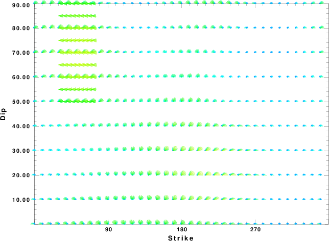
Focal mechanism sensitivity at the preferred depth. The red color indicates a very good fit to the waveforms.
Each solution is plotted as a vector at a given value of strike and dip with the angle of the vector representing the rake angle, measured, with respect to the upward vertical (N) in the figure.
|
A check on the assumed source location is possible by looking at the time shifts between the observed and predicted traces. The time shifts for waveform matching arise for several reasons:
- The origin time and epicentral distance are incorrect
- The velocity model used for the inversion is incorrect
- The velocity model used to define the P-arrival time is not the
same as the velocity model used for the waveform inversion
(assuming that the initial trace alignment is based on the
P arrival time)
Assuming only a mislocation, the time shifts are fit to a functional form:
Time_shift = A + B cos Azimuth + C Sin Azimuth
The time shifts for this inversion lead to the next figure:
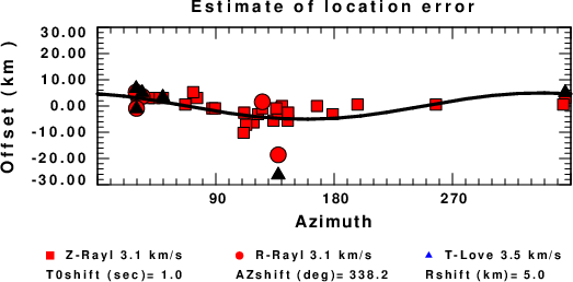
The derived shift in origin time and epicentral coordinates are given at the bottom of the figure.
Velocity Model
The WUS.model used for the waveform synthetic seismograms and for the surface wave eigenfunctions and dispersion is as follows
(The format is in the model96 format of Computer Programs in Seismology).
MODEL.01
Model after     8 iterations
ISOTROPIC
KGS
FLAT EARTH
1-D
CONSTANT VELOCITY
LINE08
LINE09
LINE10
LINE11
      H(KM)   VP(KM/S)   VS(KM/S) RHO(GM/CC)         QP         QS       ETAP       ETAS      FREFP      FREFS
     1.9000     3.4065     2.0089     2.2150  0.302E-02  0.679E-02   0.00       0.00       1.00       1.00
     6.1000     5.5445     3.2953     2.6089  0.349E-02  0.784E-02   0.00       0.00       1.00       1.00
    13.0000     6.2708     3.7396     2.7812  0.212E-02  0.476E-02   0.00       0.00       1.00       1.00
    19.0000     6.4075     3.7680     2.8223  0.111E-02  0.249E-02   0.00       0.00       1.00       1.00
     0.0000     7.9000     4.6200     3.2760  0.164E-10  0.370E-10   0.00       0.00       1.00       1.00
Last Changed Sat Apr 27 01:14:10 AM CDT 2024