Location
Location ANSS
The ANSS event ID is ak014cbigci8 and the event page is at
https://earthquake.usgs.gov/earthquakes/eventpage/ak014cbigci8/executive.
2014/09/25 17:51:17 61.945 -151.816 108.9 6.2 Alaska
Focal Mechanism
 USGS/SLU Moment Tensor Solution
 ENS  2014/09/25 17:51:17:0  61.94 -151.82 108.9 6.2 Alaska

 Stations used:
   AK.BAL AK.BARN AK.BPAW AK.BRLK AK.BWN AK.CCB AK.CNP AK.COLD
   AK.CRQ AK.CTG AK.DHY AK.DOT AK.EYAK AK.FID AK.GLB AK.GLI
   AK.HDA AK.HIN AK.HMT AK.KAI AK.KLU AK.KTH AK.MCAR AK.MCK
   AK.MDM AK.MESA AK.PAX AK.PPLA AK.RAG AK.RIDG AK.RND AK.SAW
   AK.SCM AK.SWD AK.TGL AK.TRF AK.VRDI AK.WAX AK.WRH AK.YAH
   AT.MENT AT.PMR AT.SVW2 AT.TTA IU.COLA TA.M24K

 Filtering commands used:
   cut a -30 a 210
   rtr
   taper w 0.1
   hp c 0.02 n 3
   lp c 0.04 n 3

 Best Fitting Double Couple
  Mo = 2.69e+25 dyne-cm
  Mw = 6.22
  Z  = 104 km
  Plane   Strike  Dip  Rake
   NP1      310    76   159
   NP2       45    70    15
  Principal Axes:
   Axis    Value   Plunge  Azimuth
    T   2.69e+25     24     266
    N   0.00e+00     65      97
    P  -2.69e+25      4     358

 Moment Tensor: (dyne-cm)
    Component   Value
       Mxx    -2.67e+25
       Mxy     2.24e+24
       Mxz    -2.51e+24
       Myy     2.22e+25
       Myz    -1.01e+25
       Mzz     4.48e+24


                     ----- P ------
                 ---------   ----------
              ----------------------------
             ------------------------------
           #####--------------------------###
          ##########---------------------#####
         ##############------------------######
        #################---------------########
        ####################----------##########
       #######################-------############
       ####   ##################----#############
       #### T ###################################
       ####   ##################----#############
        #######################-------##########
        #####################-----------########
         #################---------------######
          ##############------------------####
           ##########----------------------##
             ###---------------------------
              ----------------------------
                 ----------------------
                     --------------


 Global CMT Convention Moment Tensor:
      R          T          P
  4.48e+24  -2.51e+24   1.01e+25
 -2.51e+24  -2.67e+25  -2.24e+24
  1.01e+25  -2.24e+24   2.22e+25


Details of the solution is found at

http://www.eas.slu.edu/eqc/eqc_mt/MECH.NA/20140925175117/index.html
|
Preferred Solution
The preferred solution from an analysis of the surface-wave spectral amplitude radiation pattern, waveform inversion or first motion observations is
      STK = 45
      DIP = 70
     RAKE = 15
       MW = 6.22
       HS = 104.0
The NDK file is 20140925175117.ndk
The waveform inversion is preferred.
Moment Tensor Comparison
The following compares this source inversion to those provided by others. The purpose is to look for major differences and also to note slight differences that might be inherent to the processing procedure. For completeness the USGS/SLU solution is repeated from above.
| SLU |
USGSMT |
GCMT |
 USGS/SLU Moment Tensor Solution
 ENS  2014/09/25 17:51:17:0  61.94 -151.82 108.9 6.2 Alaska

 Stations used:
   AK.BAL AK.BARN AK.BPAW AK.BRLK AK.BWN AK.CCB AK.CNP AK.COLD
   AK.CRQ AK.CTG AK.DHY AK.DOT AK.EYAK AK.FID AK.GLB AK.GLI
   AK.HDA AK.HIN AK.HMT AK.KAI AK.KLU AK.KTH AK.MCAR AK.MCK
   AK.MDM AK.MESA AK.PAX AK.PPLA AK.RAG AK.RIDG AK.RND AK.SAW
   AK.SCM AK.SWD AK.TGL AK.TRF AK.VRDI AK.WAX AK.WRH AK.YAH
   AT.MENT AT.PMR AT.SVW2 AT.TTA IU.COLA TA.M24K

 Filtering commands used:
   cut a -30 a 210
   rtr
   taper w 0.1
   hp c 0.02 n 3
   lp c 0.04 n 3

 Best Fitting Double Couple
  Mo = 2.69e+25 dyne-cm
  Mw = 6.22
  Z  = 104 km
  Plane   Strike  Dip  Rake
   NP1      310    76   159
   NP2       45    70    15
  Principal Axes:
   Axis    Value   Plunge  Azimuth
    T   2.69e+25     24     266
    N   0.00e+00     65      97
    P  -2.69e+25      4     358

 Moment Tensor: (dyne-cm)
    Component   Value
       Mxx    -2.67e+25
       Mxy     2.24e+24
       Mxz    -2.51e+24
       Myy     2.22e+25
       Myz    -1.01e+25
       Mzz     4.48e+24


                     ----- P ------
                 ---------   ----------
              ----------------------------
             ------------------------------
           #####--------------------------###
          ##########---------------------#####
         ##############------------------######
        #################---------------########
        ####################----------##########
       #######################-------############
       ####   ##################----#############
       #### T ###################################
       ####   ##################----#############
        #######################-------##########
        #####################-----------########
         #################---------------######
          ##############------------------####
           ##########----------------------##
             ###---------------------------
              ----------------------------
                 ----------------------
                     --------------


 Global CMT Convention Moment Tensor:
      R          T          P
  4.48e+24  -2.51e+24   1.01e+25
 -2.51e+24  -2.67e+25  -2.24e+24
  1.01e+25  -2.24e+24   2.22e+25


Details of the solution is found at

http://www.eas.slu.edu/eqc/eqc_mt/MECH.NA/20140925175117/index.html
|
| Method Mw H (km) S1, D1, R1 S2, D2, R2 Catalog Source us
|
| Mwr 6.3 100.0 km 310, 76, 161 45, 72, 15 us us us
|

|
| Mwb 6.3 102.0 km 303, 73, 160 39, 71, 18 us us us
|

|
|
Mww 6.3 110.5 km 46, 79, 13 314, 77, 169 us us us
|

|
|
Mwc 6.3 111.6 km 315, 82, 164 47, 75, 9 gcmt gcmt us
|

|
|
CENTROID-MOMENT-TENSOR  SOLUTION
GCMT EVENT:     C201409251751A
DATA: II LD IU G  DK CU MN IC GE
 XF KP
L.P.BODY WAVES:179S, 431C, T= 40
MANTLE WAVES:  144S, 244C, T=125
SURFACE WAVES: 177S, 419C, T= 50
TIMESTAMP:      Q-20140926082604
CENTROID LOCATION:
ORIGIN TIME:      17:51:22.7 0.1
LAT:62.02N 0.00;LON:151.80W 0.01
DEP:111.6  0.3;TRIANG HDUR:  3.5
MOMENT TENSOR: SCALE 10**25 D-CM
RR= 0.274 0.013; TT=-3.560 0.016
PP= 3.280 0.016; RT=-0.299 0.012
RP= 1.000 0.011; TP= 0.139 0.014
PRINCIPAL AXES:
1.(T) VAL=  3.583;PLG=17;AZM=270
2.(N)       0.002;    72;    108
3.(P)      -3.590;     5;      2
BEST DBLE.COUPLE:M0= 3.59*10**25
NP1: STRIKE= 47;DIP=75;SLIP=   9
NP2: STRIKE=315;DIP=82;SLIP= 164

            ----- P ---
        ---------   -------
      -----------------------
    ####---------------------##
   ########-----------------####
  ###########--------------######
  #############-----------#######
 #   ############-------##########
 # T ##############----###########
 #   #############################
 ##################---############
  ###############-------#########
  #############-----------#######
   #########---------------#####
    ####--------------------###
      -----------------------
        -------------------
            -----------
|
Magnitudes
Given the availability of digital waveforms for determination of the moment tensor, this section documents the added processing leading to mLg, if appropriate to the region, and ML by application of the respective IASPEI formulae. As a research study, the linear distance term of the IASPEI formula
for ML is adjusted to remove a linear distance trend in residuals to give a regionally defined ML. The defined ML uses horizontal component recordings, but the same procedure is applied to the vertical components since there may be some interest in vertical component ground motions. Residual plots versus distance may indicate interesting features of ground motion scaling in some distance ranges. A residual plot of the regionalized magnitude is given as a function of distance and azimuth, since data sets may transcend different wave propagation provinces.
ML Magnitude
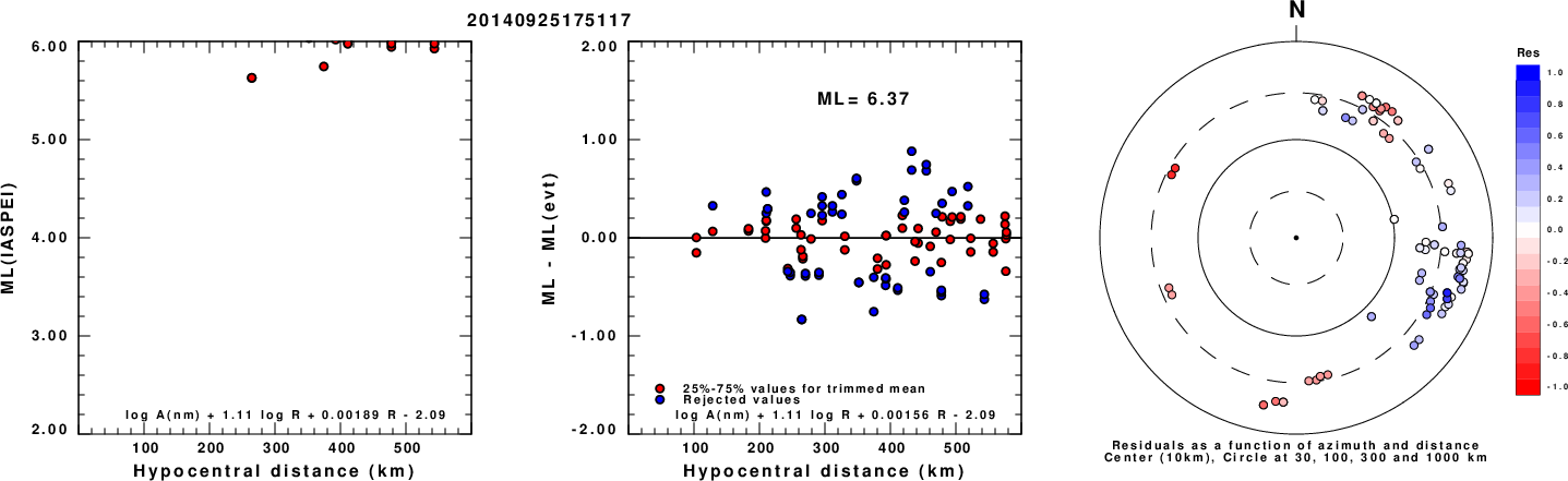
Left: ML computed using the IASPEI formula for Horizontal components. Center: ML residuals computed using a modified IASPEI formula that accounts for path specific attenuation; the values used for the trimmed mean are indicated. The ML relation used for each figure is given at the bottom of each plot.
Right: Residuals from new relation as a function of distance and azimuth.
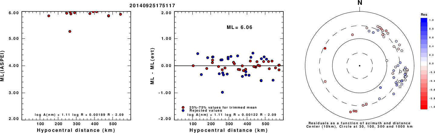
Left: ML computed using the IASPEI formula for Vertical components (research). Center: ML residuals computed using a modified IASPEI formula that accounts for path specific attenuation; the values used for the trimmed mean are indicated. The ML relation used for each figure is given at the bottom of each plot.
Right: Residuals from new relation as a function of distance and azimuth.
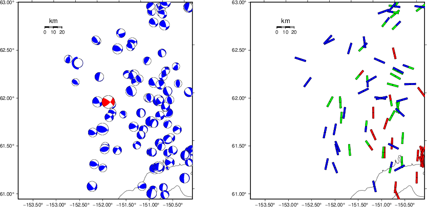
Context
The left panel of the next figure presents the focal mechanism for this earthquake (red) in the context of other nearby events (blue) in the SLU Moment Tensor Catalog. The right panel shows the inferred direction of maximum compressive stress and the type of faulting (green is strike-slip, red is normal, blue is thrust; oblique is shown by a combination of colors). Thus context plot is useful for assessing the appropriateness of the moment tensor of this event.
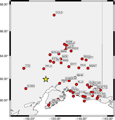
Waveform Inversion using wvfgrd96
The focal mechanism was determined using broadband seismic waveforms. The location of the event (star) and the
stations used for (red) the waveform inversion are shown in the next figure.
|
|
Location of broadband stations used for waveform inversion
|
The program wvfgrd96 was used with good traces observed at short distance to determine the focal mechanism, depth and seismic moment. This technique requires a high quality signal and well determined velocity model for the Green's functions. To the extent that these are the quality data, this type of mechanism should be preferred over the radiation pattern technique which requires the separate step of defining the pressure and tension quadrants and the correct strike.
The observed and predicted traces are filtered using the following gsac commands:
cut a -30 a 210
rtr
taper w 0.1
hp c 0.02 n 3
lp c 0.04 n 3
The results of this grid search are as follow:
           DEPTH  STK   DIP  RAKE   MW    FIT
WVFGRD96    2.0   125    75   -35   5.44 0.2496
WVFGRD96    4.0   130    75   -20   5.47 0.2718
WVFGRD96    6.0   130    80   -10   5.49 0.2803
WVFGRD96    8.0   135    85   -10   5.55 0.2850
WVFGRD96   10.0   135    80    -5   5.57 0.2748
WVFGRD96   12.0   135    65    15   5.58 0.2606
WVFGRD96   14.0   135    65    15   5.59 0.2569
WVFGRD96   16.0   135    70    20   5.60 0.2563
WVFGRD96   18.0   135    65    15   5.61 0.2571
WVFGRD96   20.0   135    65    15   5.62 0.2587
WVFGRD96   22.0    35    65   -10   5.62 0.2610
WVFGRD96   24.0    35    60   -10   5.64 0.2698
WVFGRD96   26.0    35    65   -10   5.66 0.2789
WVFGRD96   28.0    35    65   -10   5.68 0.2893
WVFGRD96   30.0    35    65   -10   5.70 0.2998
WVFGRD96   32.0    35    65   -10   5.72 0.3112
WVFGRD96   34.0    35    65   -10   5.74 0.3245
WVFGRD96   36.0    35    70   -10   5.77 0.3395
WVFGRD96   38.0    40    75    -5   5.83 0.3611
WVFGRD96   40.0    40    70    -5   5.89 0.3895
WVFGRD96   42.0    40    70    -5   5.91 0.4075
WVFGRD96   44.0    40    70    -5   5.93 0.4257
WVFGRD96   46.0    40    75   -10   5.96 0.4450
WVFGRD96   48.0    40    75   -10   5.98 0.4644
WVFGRD96   50.0    40    75    -5   5.99 0.4838
WVFGRD96   52.0    40    75    -5   6.01 0.5037
WVFGRD96   54.0    40    75    -5   6.03 0.5230
WVFGRD96   56.0    40    75    -5   6.04 0.5419
WVFGRD96   58.0    40    75    -5   6.06 0.5600
WVFGRD96   60.0    40    75     0   6.07 0.5778
WVFGRD96   62.0    40    75     0   6.08 0.5951
WVFGRD96   64.0    40    75     0   6.10 0.6122
WVFGRD96   66.0    40    75     0   6.11 0.6286
WVFGRD96   68.0    40    75     5   6.12 0.6443
WVFGRD96   70.0    40    75     5   6.13 0.6614
WVFGRD96   72.0    40    75     5   6.14 0.6772
WVFGRD96   74.0    45    75     5   6.16 0.6926
WVFGRD96   76.0    45    75     5   6.17 0.7074
WVFGRD96   78.0    45    75     5   6.17 0.7208
WVFGRD96   80.0    45    75     5   6.18 0.7324
WVFGRD96   82.0    45    75    10   6.19 0.7445
WVFGRD96   84.0    45    75    10   6.19 0.7552
WVFGRD96   86.0    45    75    10   6.20 0.7644
WVFGRD96   88.0    45    70    10   6.20 0.7728
WVFGRD96   90.0    45    70    10   6.20 0.7791
WVFGRD96   92.0    45    70    10   6.21 0.7852
WVFGRD96   94.0    45    70    10   6.21 0.7900
WVFGRD96   96.0    45    70    10   6.22 0.7936
WVFGRD96   98.0    45    70    10   6.22 0.7961
WVFGRD96  100.0    45    70    15   6.22 0.7973
WVFGRD96  102.0    45    70    15   6.22 0.7986
WVFGRD96  104.0    45    70    15   6.22 0.7995
WVFGRD96  106.0    45    70    15   6.23 0.7993
WVFGRD96  108.0    45    70    15   6.23 0.7984
WVFGRD96  110.0    45    70    15   6.23 0.7960
WVFGRD96  112.0    45    70    15   6.23 0.7939
WVFGRD96  114.0    45    70    15   6.23 0.7909
WVFGRD96  116.0    45    70    15   6.23 0.7877
WVFGRD96  118.0    45    70    15   6.24 0.7839
WVFGRD96  120.0    45    70    20   6.23 0.7804
WVFGRD96  122.0    45    70    20   6.23 0.7763
WVFGRD96  124.0    45    70    20   6.23 0.7722
WVFGRD96  126.0    45    70    20   6.23 0.7678
WVFGRD96  128.0    45    70    20   6.24 0.7627
WVFGRD96  130.0    45    70    20   6.24 0.7578
WVFGRD96  132.0    45    70    20   6.24 0.7524
WVFGRD96  134.0    45    70    20   6.24 0.7468
WVFGRD96  136.0    45    70    20   6.24 0.7414
WVFGRD96  138.0    45    70    20   6.24 0.7356
The best solution is
WVFGRD96 104.0 45 70 15 6.22 0.7995
The mechanism corresponding to the best fit is
|
|
Figure 1. Waveform inversion focal mechanism
|
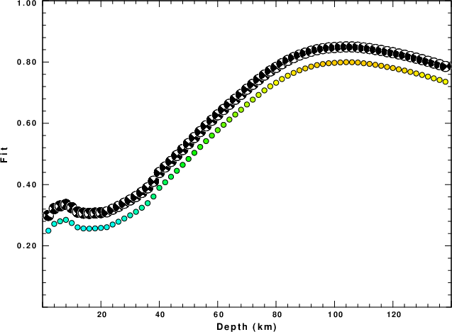
The best fit as a function of depth is given in the following figure:
|
|
Figure 2. Depth sensitivity for waveform mechanism
|
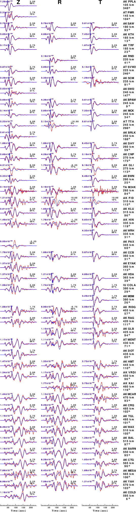
The comparison of the observed and predicted waveforms is given in the next figure. The red traces are the observed and the blue are the predicted.
Each observed-predicted component is plotted to the same scale and peak amplitudes are indicated by the numbers to the left of each trace. A pair of numbers is given in black at the right of each predicted traces. The upper number it the time shift required for maximum correlation between the observed and predicted traces. This time shift is required because the synthetics are not computed at exactly the same distance as the observed, the velocity model used in the predictions may not be perfect and the epicentral parameters may be be off.
A positive time shift indicates that the prediction is too fast and should be delayed to match the observed trace (shift to the right in this figure). A negative value indicates that the prediction is too slow. The lower number gives the percentage of variance reduction to characterize the individual goodness of fit (100% indicates a perfect fit).
The bandpass filter used in the processing and for the display was
cut a -30 a 210
rtr
taper w 0.1
hp c 0.02 n 3
lp c 0.04 n 3
|
|
Figure 3. Waveform comparison for selected depth. Red: observed; Blue - predicted. The time shift with respect to the model prediction is indicated. The percent of fit is also indicated. The time scale is relative to the first trace sample.
|
|
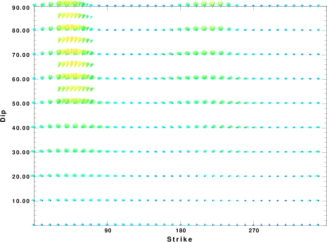
|
Focal mechanism sensitivity at the preferred depth. The red color indicates a very good fit to the waveforms.
Each solution is plotted as a vector at a given value of strike and dip with the angle of the vector representing the rake angle, measured, with respect to the upward vertical (N) in the figure.
|
A check on the assumed source location is possible by looking at the time shifts between the observed and predicted traces. The time shifts for waveform matching arise for several reasons:
- The origin time and epicentral distance are incorrect
- The velocity model used for the inversion is incorrect
- The velocity model used to define the P-arrival time is not the
same as the velocity model used for the waveform inversion
(assuming that the initial trace alignment is based on the
P arrival time)
Assuming only a mislocation, the time shifts are fit to a functional form:
Time_shift = A + B cos Azimuth + C Sin Azimuth
The time shifts for this inversion lead to the next figure:
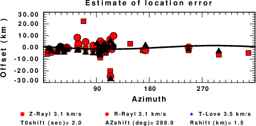
The derived shift in origin time and epicentral coordinates are given at the bottom of the figure.
Velocity Model
The WUS.model used for the waveform synthetic seismograms and for the surface wave eigenfunctions and dispersion is as follows
(The format is in the model96 format of Computer Programs in Seismology).
MODEL.01
Model after     8 iterations
ISOTROPIC
KGS
FLAT EARTH
1-D
CONSTANT VELOCITY
LINE08
LINE09
LINE10
LINE11
      H(KM)   VP(KM/S)   VS(KM/S) RHO(GM/CC)         QP         QS       ETAP       ETAS      FREFP      FREFS
     1.9000     3.4065     2.0089     2.2150  0.302E-02  0.679E-02   0.00       0.00       1.00       1.00
     6.1000     5.5445     3.2953     2.6089  0.349E-02  0.784E-02   0.00       0.00       1.00       1.00
    13.0000     6.2708     3.7396     2.7812  0.212E-02  0.476E-02   0.00       0.00       1.00       1.00
    19.0000     6.4075     3.7680     2.8223  0.111E-02  0.249E-02   0.00       0.00       1.00       1.00
     0.0000     7.9000     4.6200     3.2760  0.164E-10  0.370E-10   0.00       0.00       1.00       1.00
Last Changed Sat Apr 27 12:50:49 AM CDT 2024