Location
Location ANSS
The ANSS event ID is ak014768f0z7 and the event page is at
https://earthquake.usgs.gov/earthquakes/eventpage/ak014768f0z7/executive.
2014/06/05 14:41:14 62.842 -149.405 78.8 3.9 Arkansas
Focal Mechanism
 USGS/SLU Moment Tensor Solution
 ENS  2014/06/05 14:41:14:0  62.84 -149.40  78.8 3.9 Arkansas

 Stations used:
   AK.CCB AK.DHY AK.GHO AK.GLI AK.HARP AK.HDA AK.KTH AK.MCK
   AK.PPLA AK.RC01 AK.RIDG AK.RND AK.SAW AK.SCM AK.TRF AK.WRH
   AT.PMR IM.IL31 IU.COLA

 Filtering commands used:
   cut a -30 a 100
   rtr
   taper w 0.1
   hp c 0.02 n 3
   lp c 0.06 n 3

 Best Fitting Double Couple
  Mo = 1.02e+22 dyne-cm
  Mw = 3.94
  Z  = 89 km
  Plane   Strike  Dip  Rake
   NP1       85    90   -10
   NP2      175    80   -180
  Principal Axes:
   Axis    Value   Plunge  Azimuth
    T   1.02e+22      7     130
    N   0.00e+00     80     265
    P  -1.02e+22      7      40

 Moment Tensor: (dyne-cm)
    Component   Value
       Mxx    -1.75e+21
       Mxy    -9.92e+21
       Mxz    -1.77e+21
       Myy     1.75e+21
       Myz     1.55e+20
       Mzz     1.55e+14


                     #####---------
                 #########------------
              ###########------------- P -
             ############-------------   --
           ##############--------------------
          ###############---------------------
         ################----------------------
        #################-----------------------
        #################-----------------------
       ##################------------------------
       ##################--------------##########
       ##########---------#######################
       -------------------#######################
        ------------------######################
        ------------------######################
         -----------------#####################
          -----------------###############   #
           ----------------############### T
             ---------------##############
              --------------##############
                 ------------##########
                     --------######


 Global CMT Convention Moment Tensor:
      R          T          P
  1.55e+14  -1.77e+21  -1.55e+20
 -1.77e+21  -1.75e+21   9.92e+21
 -1.55e+20   9.92e+21   1.75e+21


Details of the solution is found at

http://www.eas.slu.edu/eqc/eqc_mt/MECH.NA/20140605144114/index.html
|
Preferred Solution
The preferred solution from an analysis of the surface-wave spectral amplitude radiation pattern, waveform inversion or first motion observations is
      STK = 85
      DIP = 90
     RAKE = -10
       MW = 3.94
       HS = 89.0
The NDK file is 20140605144114.ndk
The waveform inversion is preferred.
Magnitudes
Given the availability of digital waveforms for determination of the moment tensor, this section documents the added processing leading to mLg, if appropriate to the region, and ML by application of the respective IASPEI formulae. As a research study, the linear distance term of the IASPEI formula
for ML is adjusted to remove a linear distance trend in residuals to give a regionally defined ML. The defined ML uses horizontal component recordings, but the same procedure is applied to the vertical components since there may be some interest in vertical component ground motions. Residual plots versus distance may indicate interesting features of ground motion scaling in some distance ranges. A residual plot of the regionalized magnitude is given as a function of distance and azimuth, since data sets may transcend different wave propagation provinces.
ML Magnitude
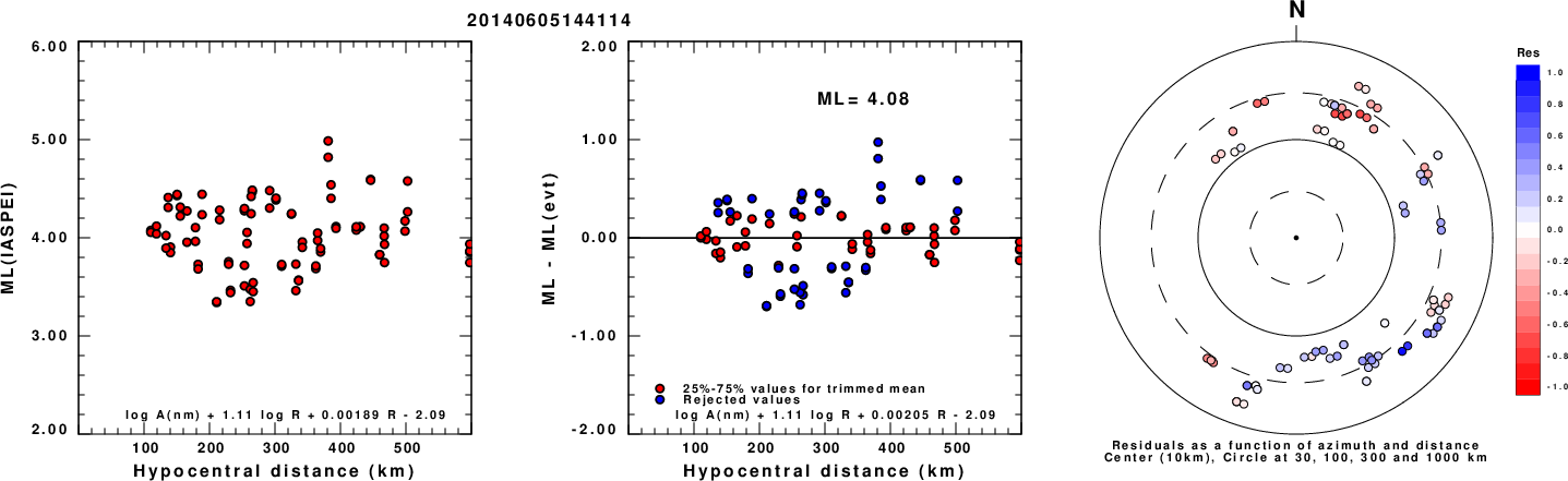
Left: ML computed using the IASPEI formula for Horizontal components. Center: ML residuals computed using a modified IASPEI formula that accounts for path specific attenuation; the values used for the trimmed mean are indicated. The ML relation used for each figure is given at the bottom of each plot.
Right: Residuals from new relation as a function of distance and azimuth.
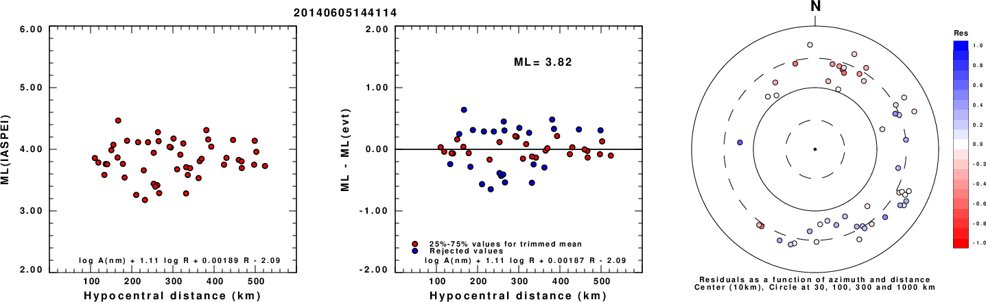
Left: ML computed using the IASPEI formula for Vertical components (research). Center: ML residuals computed using a modified IASPEI formula that accounts for path specific attenuation; the values used for the trimmed mean are indicated. The ML relation used for each figure is given at the bottom of each plot.
Right: Residuals from new relation as a function of distance and azimuth.
Context
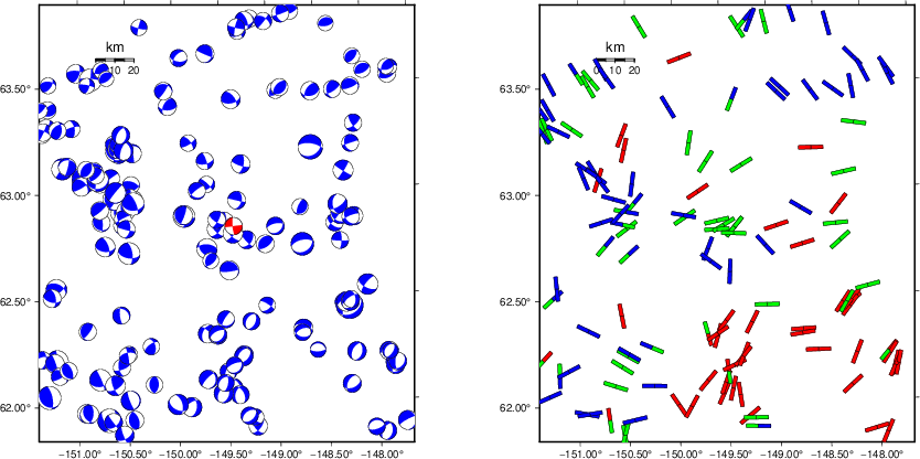
The left panel of the next figure presents the focal mechanism for this earthquake (red) in the context of other nearby events (blue) in the SLU Moment Tensor Catalog. The right panel shows the inferred direction of maximum compressive stress and the type of faulting (green is strike-slip, red is normal, blue is thrust; oblique is shown by a combination of colors). Thus context plot is useful for assessing the appropriateness of the moment tensor of this event.
Waveform Inversion using wvfgrd96
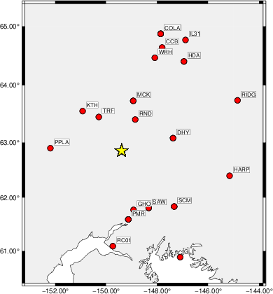
The focal mechanism was determined using broadband seismic waveforms. The location of the event (star) and the
stations used for (red) the waveform inversion are shown in the next figure.
|
|
Location of broadband stations used for waveform inversion
|
The program wvfgrd96 was used with good traces observed at short distance to determine the focal mechanism, depth and seismic moment. This technique requires a high quality signal and well determined velocity model for the Green's functions. To the extent that these are the quality data, this type of mechanism should be preferred over the radiation pattern technique which requires the separate step of defining the pressure and tension quadrants and the correct strike.
The observed and predicted traces are filtered using the following gsac commands:
cut a -30 a 100
rtr
taper w 0.1
hp c 0.02 n 3
lp c 0.06 n 3
The results of this grid search are as follow:
           DEPTH  STK   DIP  RAKE   MW    FIT
WVFGRD96    2.0    -5    80    -5   3.16 0.3248
WVFGRD96    4.0    -5    80    -5   3.24 0.3712
WVFGRD96    6.0   355    80   -15   3.30 0.3856
WVFGRD96    8.0   355    75   -15   3.35 0.3935
WVFGRD96    9.0   265    85    -5   3.36 0.4051
WVFGRD96   10.0    85    90     5   3.38 0.4164
WVFGRD96   12.0    85    90     5   3.42 0.4303
WVFGRD96   14.0   265    85    -5   3.44 0.4390
WVFGRD96   16.0   265    90     0   3.47 0.4466
WVFGRD96   18.0    85    90     0   3.49 0.4532
WVFGRD96   19.0   265    85    -5   3.50 0.4592
WVFGRD96   20.0   265    85    -5   3.51 0.4639
WVFGRD96   22.0   265    75     5   3.53 0.4743
WVFGRD96   24.0   265    75     5   3.55 0.4856
WVFGRD96   26.0   265    75     5   3.56 0.4952
WVFGRD96   28.0   265    75     5   3.58 0.5025
WVFGRD96   29.0   265    80    10   3.59 0.5070
WVFGRD96   30.0   270    80    10   3.60 0.5111
WVFGRD96   32.0   270    80    10   3.62 0.5181
WVFGRD96   34.0   265    80    10   3.64 0.5231
WVFGRD96   36.0   265    80    10   3.66 0.5263
WVFGRD96   38.0   265    90     5   3.70 0.5341
WVFGRD96   39.0   265    90     5   3.71 0.5398
WVFGRD96   40.0   265    90     5   3.73 0.5458
WVFGRD96   42.0   270    80    10   3.76 0.5428
WVFGRD96   44.0   270    80    10   3.77 0.5431
WVFGRD96   46.0    85    80   -10   3.79 0.5478
WVFGRD96   48.0    85    80   -10   3.80 0.5539
WVFGRD96   49.0    85    80   -10   3.81 0.5575
WVFGRD96   50.0    85    80   -10   3.81 0.5614
WVFGRD96   52.0    85    80   -10   3.83 0.5691
WVFGRD96   54.0    85    80   -10   3.84 0.5770
WVFGRD96   56.0    85    80   -10   3.85 0.5854
WVFGRD96   58.0    85    80   -15   3.86 0.5930
WVFGRD96   59.0    85    85   -10   3.86 0.5962
WVFGRD96   60.0    85    85   -10   3.86 0.6004
WVFGRD96   62.0    85    85   -10   3.87 0.6071
WVFGRD96   64.0    85    85   -10   3.88 0.6137
WVFGRD96   66.0    85    85   -10   3.88 0.6190
WVFGRD96   68.0    85    85   -10   3.89 0.6245
WVFGRD96   69.0   265    90    10   3.89 0.6246
WVFGRD96   70.0    85    85   -10   3.89 0.6285
WVFGRD96   72.0    85    85   -10   3.90 0.6317
WVFGRD96   74.0   265    90    10   3.91 0.6349
WVFGRD96   76.0    85    90   -10   3.91 0.6378
WVFGRD96   78.0    85    90   -10   3.92 0.6397
WVFGRD96   79.0    85    90   -10   3.92 0.6408
WVFGRD96   80.0    85    90   -10   3.92 0.6422
WVFGRD96   82.0    85    90   -10   3.92 0.6431
WVFGRD96   84.0    85    90   -10   3.93 0.6441
WVFGRD96   86.0    85    90   -10   3.93 0.6451
WVFGRD96   88.0    85    90   -10   3.94 0.6453
WVFGRD96   89.0    85    90   -10   3.94 0.6455
WVFGRD96   90.0    85    90   -10   3.94 0.6453
WVFGRD96   92.0    85    90   -10   3.95 0.6444
WVFGRD96   94.0    85    90   -10   3.95 0.6439
WVFGRD96   96.0   265    85    10   3.96 0.6445
WVFGRD96   98.0    85    90   -10   3.96 0.6433
WVFGRD96   99.0   265    85    10   3.96 0.6436
WVFGRD96  100.0   265    85    10   3.97 0.6440
WVFGRD96  102.0    85    90   -10   3.97 0.6413
WVFGRD96  104.0    85    90   -10   3.97 0.6399
WVFGRD96  106.0    85    90    -5   3.97 0.6385
WVFGRD96  108.0    85    90    -5   3.97 0.6370
WVFGRD96  109.0   265    85     5   3.98 0.6384
WVFGRD96  110.0    85    90    -5   3.98 0.6353
WVFGRD96  112.0    85    90    -5   3.98 0.6333
WVFGRD96  114.0    85    90    -5   3.99 0.6323
WVFGRD96  116.0    85    90    -5   3.99 0.6310
WVFGRD96  118.0    85    90    -5   3.99 0.6292
WVFGRD96  119.0   265    85     5   4.00 0.6310
The best solution is
WVFGRD96 89.0 85 90 -10 3.94 0.6455
The mechanism corresponding to the best fit is
|
|
Figure 1. Waveform inversion focal mechanism
|
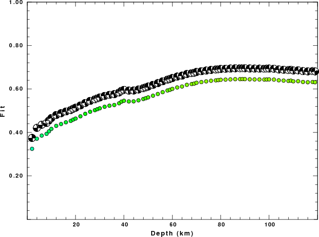
The best fit as a function of depth is given in the following figure:
|
|
Figure 2. Depth sensitivity for waveform mechanism
|
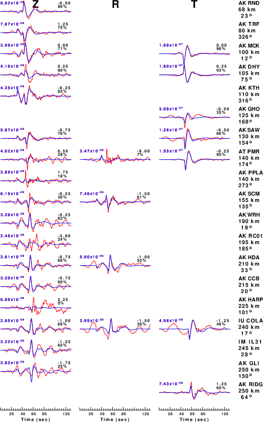
The comparison of the observed and predicted waveforms is given in the next figure. The red traces are the observed and the blue are the predicted.
Each observed-predicted component is plotted to the same scale and peak amplitudes are indicated by the numbers to the left of each trace. A pair of numbers is given in black at the right of each predicted traces. The upper number it the time shift required for maximum correlation between the observed and predicted traces. This time shift is required because the synthetics are not computed at exactly the same distance as the observed, the velocity model used in the predictions may not be perfect and the epicentral parameters may be be off.
A positive time shift indicates that the prediction is too fast and should be delayed to match the observed trace (shift to the right in this figure). A negative value indicates that the prediction is too slow. The lower number gives the percentage of variance reduction to characterize the individual goodness of fit (100% indicates a perfect fit).
The bandpass filter used in the processing and for the display was
cut a -30 a 100
rtr
taper w 0.1
hp c 0.02 n 3
lp c 0.06 n 3
|
|
Figure 3. Waveform comparison for selected depth. Red: observed; Blue - predicted. The time shift with respect to the model prediction is indicated. The percent of fit is also indicated. The time scale is relative to the first trace sample.
|
|
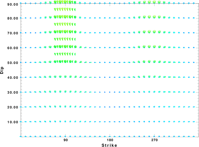
|
Focal mechanism sensitivity at the preferred depth. The red color indicates a very good fit to the waveforms.
Each solution is plotted as a vector at a given value of strike and dip with the angle of the vector representing the rake angle, measured, with respect to the upward vertical (N) in the figure.
|
A check on the assumed source location is possible by looking at the time shifts between the observed and predicted traces. The time shifts for waveform matching arise for several reasons:
- The origin time and epicentral distance are incorrect
- The velocity model used for the inversion is incorrect
- The velocity model used to define the P-arrival time is not the
same as the velocity model used for the waveform inversion
(assuming that the initial trace alignment is based on the
P arrival time)
Assuming only a mislocation, the time shifts are fit to a functional form:
Time_shift = A + B cos Azimuth + C Sin Azimuth
The time shifts for this inversion lead to the next figure:
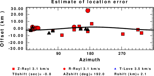
The derived shift in origin time and epicentral coordinates are given at the bottom of the figure.
Velocity Model
The WUS.model used for the waveform synthetic seismograms and for the surface wave eigenfunctions and dispersion is as follows
(The format is in the model96 format of Computer Programs in Seismology).
MODEL.01
Model after     8 iterations
ISOTROPIC
KGS
FLAT EARTH
1-D
CONSTANT VELOCITY
LINE08
LINE09
LINE10
LINE11
      H(KM)   VP(KM/S)   VS(KM/S) RHO(GM/CC)         QP         QS       ETAP       ETAS      FREFP      FREFS
     1.9000     3.4065     2.0089     2.2150  0.302E-02  0.679E-02   0.00       0.00       1.00       1.00
     6.1000     5.5445     3.2953     2.6089  0.349E-02  0.784E-02   0.00       0.00       1.00       1.00
    13.0000     6.2708     3.7396     2.7812  0.212E-02  0.476E-02   0.00       0.00       1.00       1.00
    19.0000     6.4075     3.7680     2.8223  0.111E-02  0.249E-02   0.00       0.00       1.00       1.00
     0.0000     7.9000     4.6200     3.2760  0.164E-10  0.370E-10   0.00       0.00       1.00       1.00
Last Changed Fri Apr 26 07:43:28 PM CDT 2024