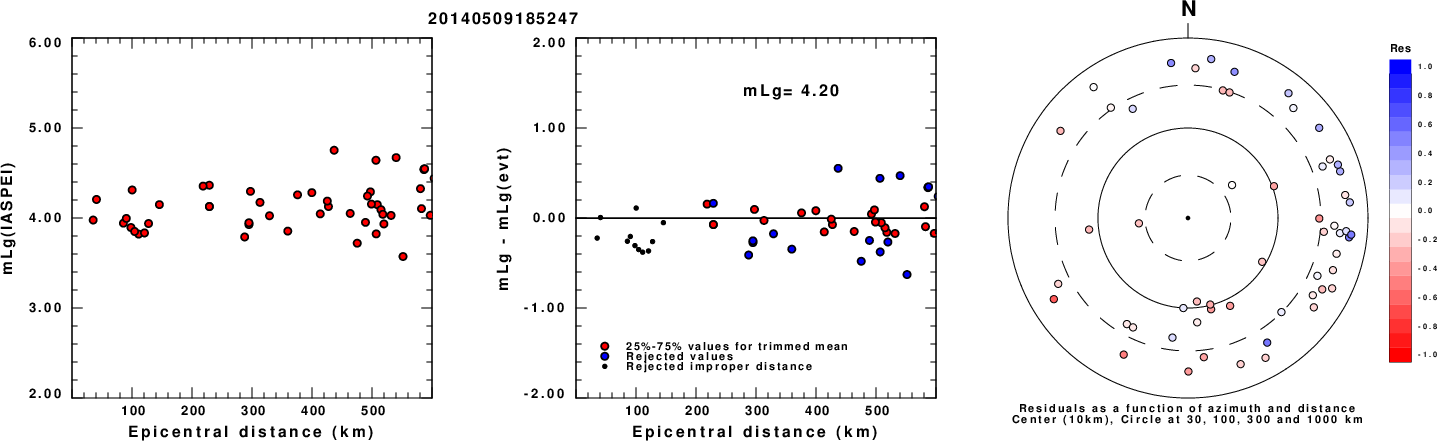
Left: mLg computed using the IASPEI formula. Center: mLg residuals versus epicentral distance ; the values used for the trimmed mean magnitude estimate are indicated. Right: residuals as a function of distance and azimuth.
The ANSS event ID is usb000qfz9 and the event page is at https://earthquake.usgs.gov/earthquakes/eventpage/usb000qfz9/executive.
2014/05/09 18:52:47 36.583 -97.618 4.0 3.9 Oklahoma
 USGS/SLU Moment Tensor Solution
 ENS  2014/05/09 18:52:47:0  36.58  -97.62   4.0 3.9 Oklahoma

 Stations used:
   AG.FCAR AG.HHAR AG.LCAR AG.WHAR AG.WLAR GS.OK025 GS.OK027
   GS.OK028 GS.OK029 IU.CCM N4.N33B N4.N35B N4.P38B N4.P40B
   N4.R32B N4.R40B N4.S39B N4.T35B N4.T42B N4.U38B N4.Z35B
   N4.Z38B NM.UALR OK.BCOK OK.FNO OK.U32A OK.X37A TA.ABTX
   TA.KSCO TA.U40A TA.W39A TA.WHTX TA.X40A US.AMTX US.CBKS
   US.KSU1 US.MIAR US.WMOK

 Filtering commands used:
   cut a -30 a 180
   rtr
   taper w 0.1
   hp c 0.03 n 3
   lp c 0.06 n 3

 Best Fitting Double Couple
  Mo = 7.50e+21 dyne-cm
  Mw = 3.85
  Z  = 4 km
  Plane   Strike  Dip  Rake
   NP1      360    90   -10
   NP2       90    80   -180
  Principal Axes:
   Axis    Value   Plunge  Azimuth
    T   7.50e+21      7      45
    N   0.00e+00     80     180
    P  -7.50e+21      7     315

 Moment Tensor: (dyne-cm)
    Component   Value
       Mxx    -0.00e+00
       Mxy     7.39e+21
       Mxz     3.23e+14
       Myy    -1.14e+14
       Myz     1.30e+21
       Mzz     1.14e+14


                     -------#######
                 -----------###########
                ------------############
              P ------------############ T
           --   ------------############   ##
          ------------------##################
         -------------------###################
        --------------------####################
        --------------------####################
       ---------------------#####################
       ---------------------#####################
       ###------------------##################---
       #####################---------------------
        ####################--------------------
        ####################--------------------
         ###################-------------------
          ##################------------------
           #################-----------------
             ###############---------------
              ##############--------------
                 ###########-----------
                     #######-------


 Global CMT Convention Moment Tensor:
      R          T          P
  1.14e+14   3.23e+14  -1.30e+21
  3.23e+14  -0.00e+00  -7.39e+21
 -1.30e+21  -7.39e+21  -1.14e+14


Details of the solution is found at

http://www.eas.slu.edu/eqc/eqc_mt/MECH.NA/20140509185247/index.html
|
      STK = 0
      DIP = 90
     RAKE = -10
       MW = 3.85
       HS = 4.0
The NDK file is 20140509185247.ndk The waveform inversion is preferred.
The following compares this source inversion to those provided by others. The purpose is to look for major differences and also to note slight differences that might be inherent to the processing procedure. For completeness the USGS/SLU solution is repeated from above.
 USGS/SLU Moment Tensor Solution
 ENS  2014/05/09 18:52:47:0  36.58  -97.62   4.0 3.9 Oklahoma

 Stations used:
   AG.FCAR AG.HHAR AG.LCAR AG.WHAR AG.WLAR GS.OK025 GS.OK027
   GS.OK028 GS.OK029 IU.CCM N4.N33B N4.N35B N4.P38B N4.P40B
   N4.R32B N4.R40B N4.S39B N4.T35B N4.T42B N4.U38B N4.Z35B
   N4.Z38B NM.UALR OK.BCOK OK.FNO OK.U32A OK.X37A TA.ABTX
   TA.KSCO TA.U40A TA.W39A TA.WHTX TA.X40A US.AMTX US.CBKS
   US.KSU1 US.MIAR US.WMOK

 Filtering commands used:
   cut a -30 a 180
   rtr
   taper w 0.1
   hp c 0.03 n 3
   lp c 0.06 n 3

 Best Fitting Double Couple
  Mo = 7.50e+21 dyne-cm
  Mw = 3.85
  Z  = 4 km
  Plane   Strike  Dip  Rake
   NP1      360    90   -10
   NP2       90    80   -180
  Principal Axes:
   Axis    Value   Plunge  Azimuth
    T   7.50e+21      7      45
    N   0.00e+00     80     180
    P  -7.50e+21      7     315

 Moment Tensor: (dyne-cm)
    Component   Value
       Mxx    -0.00e+00
       Mxy     7.39e+21
       Mxz     3.23e+14
       Myy    -1.14e+14
       Myz     1.30e+21
       Mzz     1.14e+14


                     -------#######
                 -----------###########
                ------------############
              P ------------############ T
           --   ------------############   ##
          ------------------##################
         -------------------###################
        --------------------####################
        --------------------####################
       ---------------------#####################
       ---------------------#####################
       ###------------------##################---
       #####################---------------------
        ####################--------------------
        ####################--------------------
         ###################-------------------
          ##################------------------
           #################-----------------
             ###############---------------
              ##############--------------
                 ###########-----------
                     #######-------


 Global CMT Convention Moment Tensor:
      R          T          P
  1.14e+14   3.23e+14  -1.30e+21
  3.23e+14  -0.00e+00  -7.39e+21
 -1.30e+21  -7.39e+21  -1.14e+14


Details of the solution is found at

http://www.eas.slu.edu/eqc/eqc_mt/MECH.NA/20140509185247/index.html
|
Moment magnitude derived from a moment tensor
inversion of complete waveforms at regional
distances (less than ~8 degrees), generally used
for the analysis of small to moderate size earthquakes
(typically Mw 3.5-6.0) crust or upper mantle earthquakes.

Moment
    8.75e+14 N-m
Magnitude
    3.9
Percent DC
    89%
Depth
    4.0 km
Updated
    2014-05-09 19:07:08 UTC
Author
    us
Catalog
    us
Contributor
    us
Code
    us_b000qfz9_mwr

Principal Axes
Axis	Value	Plunge	Azimuth
T	8.982	19	31
N	-0.487	52	275
P	-8.495	32	133
Nodal Planes
Plane	Strike	Dip	Rake
NP1	264	82	-142
NP2	168	53	-10
|
Given the availability of digital waveforms for determination of the moment tensor, this section documents the added processing leading to mLg, if appropriate to the region, and ML by application of the respective IASPEI formulae. As a research study, the linear distance term of the IASPEI formula for ML is adjusted to remove a linear distance trend in residuals to give a regionally defined ML. The defined ML uses horizontal component recordings, but the same procedure is applied to the vertical components since there may be some interest in vertical component ground motions. Residual plots versus distance may indicate interesting features of ground motion scaling in some distance ranges. A residual plot of the regionalized magnitude is given as a function of distance and azimuth, since data sets may transcend different wave propagation provinces.
Left: mLg computed using the IASPEI formula. Center: mLg residuals versus epicentral distance ; the values used for the trimmed mean magnitude estimate are indicated.
Right: residuals as a function of distance and azimuth.
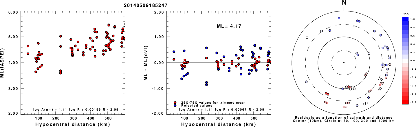
Left: ML computed using the IASPEI formula for Horizontal components. Center: ML residuals computed using a modified IASPEI formula that accounts for path specific attenuation; the values used for the trimmed mean are indicated. The ML relation used for each figure is given at the bottom of each plot.
Right: Residuals from new relation as a function of distance and azimuth.
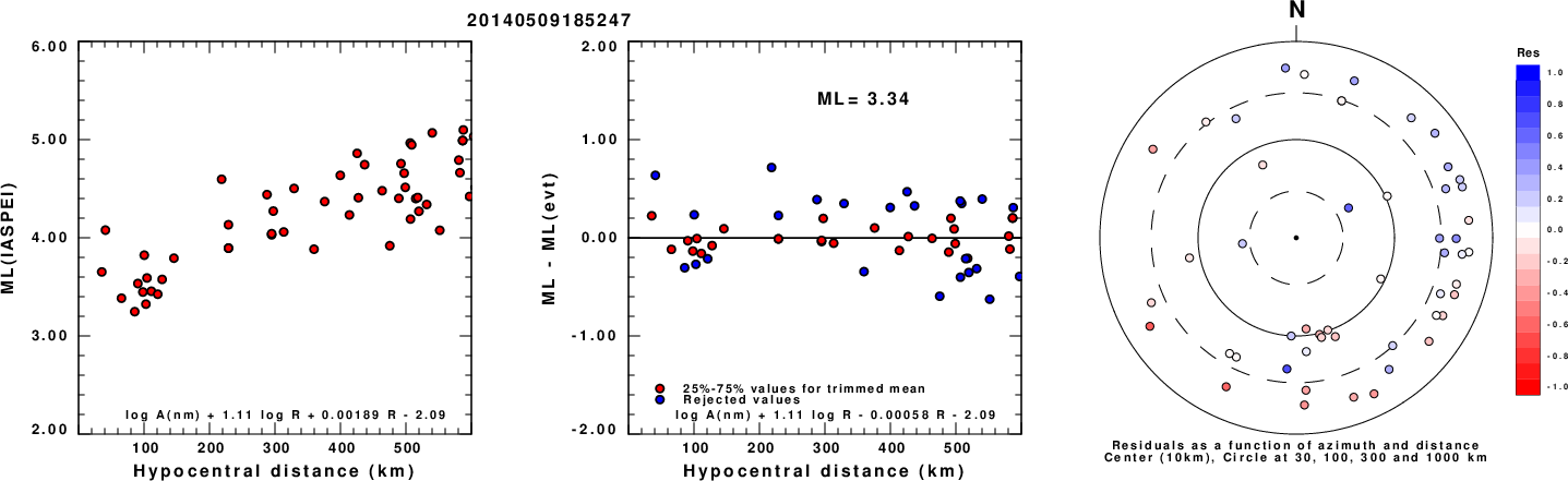
Left: ML computed using the IASPEI formula for Vertical components (research). Center: ML residuals computed using a modified IASPEI formula that accounts for path specific attenuation; the values used for the trimmed mean are indicated. The ML relation used for each figure is given at the bottom of each plot.
Right: Residuals from new relation as a function of distance and azimuth.
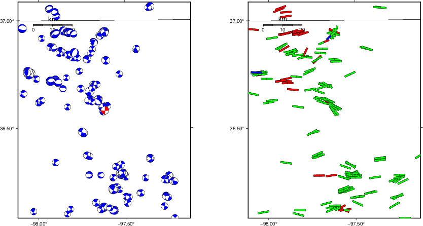 |
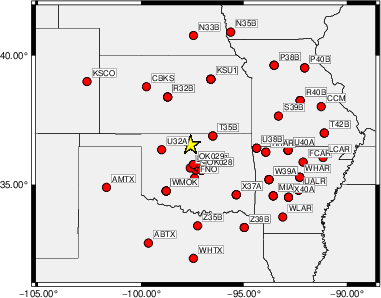
The focal mechanism was determined using broadband seismic waveforms. The location of the event (star) and the stations used for (red) the waveform inversion are shown in the next figure.
|
|
|
The program wvfgrd96 was used with good traces observed at short distance to determine the focal mechanism, depth and seismic moment. This technique requires a high quality signal and well determined velocity model for the Green's functions. To the extent that these are the quality data, this type of mechanism should be preferred over the radiation pattern technique which requires the separate step of defining the pressure and tension quadrants and the correct strike.
The observed and predicted traces are filtered using the following gsac commands:
cut a -30 a 180
rtr
taper w 0.1
hp c 0.03 n 3
lp c 0.06 n 3
The results of this grid search are as follow:
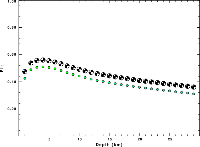
           DEPTH  STK   DIP  RAKE   MW    FIT
WVFGRD96    1.0   180    90   -10   3.70 0.4250
WVFGRD96    2.0   175    80   -15   3.79 0.4883
WVFGRD96    3.0     0    90    10   3.83 0.5062
WVFGRD96    4.0     0    90   -10   3.85 0.5097
WVFGRD96    5.0   180    90    10   3.87 0.5049
WVFGRD96    6.0     0    90   -10   3.89 0.4953
WVFGRD96    7.0     0    90   -10   3.91 0.4823
WVFGRD96    8.0     0    90    10   3.93 0.4671
WVFGRD96    9.0   180    90   -15   3.95 0.4538
WVFGRD96   10.0     0    90    15   3.96 0.4419
WVFGRD96   11.0     0    85    15   3.96 0.4304
WVFGRD96   12.0   180    90   -15   3.97 0.4196
WVFGRD96   13.0   180    90   -15   3.98 0.4097
WVFGRD96   14.0     0    85    15   3.99 0.4012
WVFGRD96   15.0     0    85    15   3.99 0.3933
WVFGRD96   16.0     0    90    15   4.00 0.3860
WVFGRD96   17.0   180    90   -15   4.01 0.3790
WVFGRD96   18.0     0    90    15   4.02 0.3721
WVFGRD96   19.0   180    90   -15   4.02 0.3655
WVFGRD96   20.0     0    90    15   4.03 0.3591
WVFGRD96   21.0   175    85   -20   4.03 0.3540
WVFGRD96   22.0     0    90    20   4.04 0.3481
WVFGRD96   23.0   175    85   -20   4.04 0.3431
WVFGRD96   24.0     0    90    20   4.06 0.3370
WVFGRD96   25.0   175    85   -20   4.05 0.3325
WVFGRD96   26.0     0    90    20   4.07 0.3263
WVFGRD96   27.0     0    90    25   4.08 0.3210
WVFGRD96   28.0   175    85   -25   4.08 0.3169
WVFGRD96   29.0     0    90    25   4.09 0.3108
The best solution is
WVFGRD96 4.0 0 90 -10 3.85 0.5097
The mechanism corresponding to the best fit is
|
|
|
The best fit as a function of depth is given in the following figure:
|
|
|
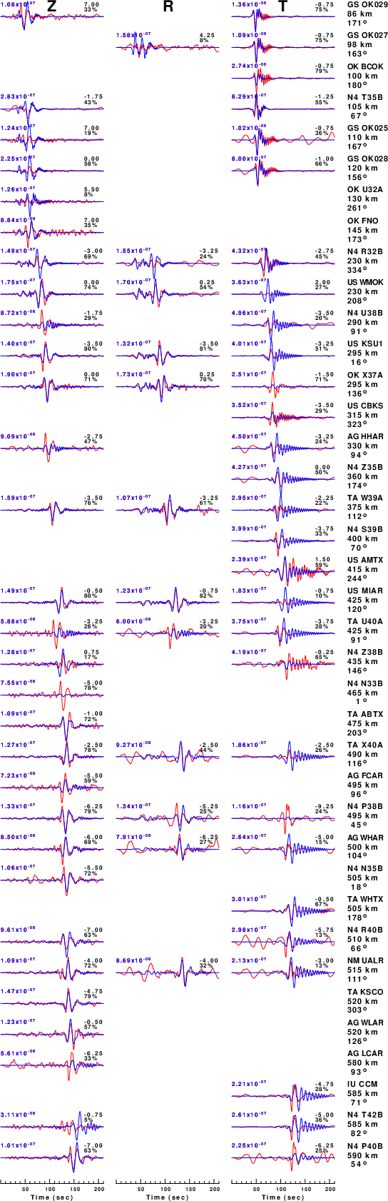
The comparison of the observed and predicted waveforms is given in the next figure. The red traces are the observed and the blue are the predicted. Each observed-predicted component is plotted to the same scale and peak amplitudes are indicated by the numbers to the left of each trace. A pair of numbers is given in black at the right of each predicted traces. The upper number it the time shift required for maximum correlation between the observed and predicted traces. This time shift is required because the synthetics are not computed at exactly the same distance as the observed, the velocity model used in the predictions may not be perfect and the epicentral parameters may be be off. A positive time shift indicates that the prediction is too fast and should be delayed to match the observed trace (shift to the right in this figure). A negative value indicates that the prediction is too slow. The lower number gives the percentage of variance reduction to characterize the individual goodness of fit (100% indicates a perfect fit).
The bandpass filter used in the processing and for the display was
cut a -30 a 180
rtr
taper w 0.1
hp c 0.03 n 3
lp c 0.06 n 3
|
| Figure 3. Waveform comparison for selected depth. Red: observed; Blue - predicted. The time shift with respect to the model prediction is indicated. The percent of fit is also indicated. The time scale is relative to the first trace sample. |
|
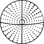
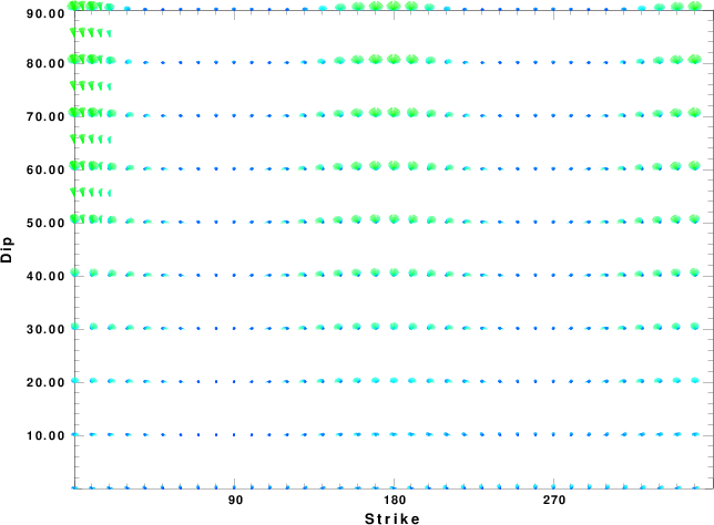
| Focal mechanism sensitivity at the preferred depth. The red color indicates a very good fit to the waveforms. Each solution is plotted as a vector at a given value of strike and dip with the angle of the vector representing the rake angle, measured, with respect to the upward vertical (N) in the figure. |
A check on the assumed source location is possible by looking at the time shifts between the observed and predicted traces. The time shifts for waveform matching arise for several reasons:
Time_shift = A + B cos Azimuth + C Sin Azimuth
The time shifts for this inversion lead to the next figure:
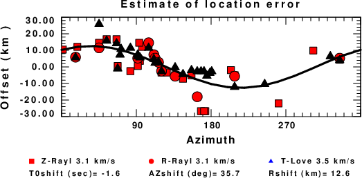
The derived shift in origin time and epicentral coordinates are given at the bottom of the figure.
The WUS.model used for the waveform synthetic seismograms and for the surface wave eigenfunctions and dispersion is as follows (The format is in the model96 format of Computer Programs in Seismology).
MODEL.01
Model after     8 iterations
ISOTROPIC
KGS
FLAT EARTH
1-D
CONSTANT VELOCITY
LINE08
LINE09
LINE10
LINE11
      H(KM)   VP(KM/S)   VS(KM/S) RHO(GM/CC)         QP         QS       ETAP       ETAS      FREFP      FREFS
     1.9000     3.4065     2.0089     2.2150  0.302E-02  0.679E-02   0.00       0.00       1.00       1.00
     6.1000     5.5445     3.2953     2.6089  0.349E-02  0.784E-02   0.00       0.00       1.00       1.00
    13.0000     6.2708     3.7396     2.7812  0.212E-02  0.476E-02   0.00       0.00       1.00       1.00
    19.0000     6.4075     3.7680     2.8223  0.111E-02  0.249E-02   0.00       0.00       1.00       1.00
     0.0000     7.9000     4.6200     3.2760  0.164E-10  0.370E-10   0.00       0.00       1.00       1.00