Location
Location ANSS
The ANSS event ID is ak0144vn0ngp and the event page is at
https://earthquake.usgs.gov/earthquakes/eventpage/ak0144vn0ngp/executive.
2014/04/16 20:24:24 62.894 -149.912 83.0 5.1 Alaska
Focal Mechanism
 USGS/SLU Moment Tensor Solution
 ENS  2014/04/16 20:24:24:0  62.89 -149.91  83.0 5.1 Alaska

 Stations used:
   AK.BARN AK.BPAW AK.BRLK AK.BWN AK.CCB AK.COLD AK.CRQ AK.CTG
   AK.DHY AK.FID AK.FYU AK.GHO AK.GLB AK.GLI AK.HDA AK.HOM
   AK.KNK AK.KTH AK.MCAR AK.MCK AK.MDM AK.MLY AK.NEA AK.PPD
   AK.PPLA AK.RC01 AK.RND AK.SAW AK.SCM AK.SKN AK.SSN AK.SWD
   AK.TGL AK.TRF AK.WRH AT.MID AT.PMR AT.SVW2 AV.RED CN.DAWY
   IM.IL31 IU.COLA

 Filtering commands used:
   cut a -30 a 180
   rtr
   taper w 0.1
   hp c 0.02 n 3
   lp c 0.06 n 3

 Best Fitting Double Couple
  Mo = 3.24e+23 dyne-cm
  Mw = 4.94
  Z  = 86 km
  Plane   Strike  Dip  Rake
   NP1      100    85    25
   NP2        8    65   174
  Principal Axes:
   Axis    Value   Plunge  Azimuth
    T   3.24e+23     21     327
    N   0.00e+00     65     111
    P  -3.24e+23     14     231

 Moment Tensor: (dyne-cm)
    Component   Value
       Mxx     7.69e+22
       Mxy    -2.79e+23
       Mxz     1.37e+23
       Myy    -1.01e+23
       Myz    -1.79e+21
       Mzz     2.37e+22


                     ###########---
                 ###############-------
              ###   #############---------
             #### T ##############---------
           ######   ##############-----------
          ########################------------
         ##########################------------
        ###########################-------------
        ###########################-------------
       ---#########################--------------
       ----------#################---------------
       -------------------########---------------
       ---------------------------####-----------
        --------------------------##############
        -------------------------###############
         ------------------------##############
          ---   ----------------##############
           -- P ---------------##############
                --------------#############
              ---------------#############
                 -----------###########
                     -----#########


 Global CMT Convention Moment Tensor:
      R          T          P
  2.37e+22   1.37e+23   1.79e+21
  1.37e+23   7.69e+22   2.79e+23
  1.79e+21   2.79e+23  -1.01e+23


Details of the solution is found at

http://www.eas.slu.edu/eqc/eqc_mt/MECH.NA/20140416202424/index.html
|
Preferred Solution
The preferred solution from an analysis of the surface-wave spectral amplitude radiation pattern, waveform inversion or first motion observations is
      STK = 100
      DIP = 85
     RAKE = 25
       MW = 4.94
       HS = 86.0
The NDK file is 20140416202424.ndk
The waveform inversion is preferred.
Moment Tensor Comparison
The following compares this source inversion to those provided by others. The purpose is to look for major differences and also to note slight differences that might be inherent to the processing procedure. For completeness the USGS/SLU solution is repeated from above.
| SLU |
USGSMT |
 USGS/SLU Moment Tensor Solution
 ENS  2014/04/16 20:24:24:0  62.89 -149.91  83.0 5.1 Alaska

 Stations used:
   AK.BARN AK.BPAW AK.BRLK AK.BWN AK.CCB AK.COLD AK.CRQ AK.CTG
   AK.DHY AK.FID AK.FYU AK.GHO AK.GLB AK.GLI AK.HDA AK.HOM
   AK.KNK AK.KTH AK.MCAR AK.MCK AK.MDM AK.MLY AK.NEA AK.PPD
   AK.PPLA AK.RC01 AK.RND AK.SAW AK.SCM AK.SKN AK.SSN AK.SWD
   AK.TGL AK.TRF AK.WRH AT.MID AT.PMR AT.SVW2 AV.RED CN.DAWY
   IM.IL31 IU.COLA

 Filtering commands used:
   cut a -30 a 180
   rtr
   taper w 0.1
   hp c 0.02 n 3
   lp c 0.06 n 3

 Best Fitting Double Couple
  Mo = 3.24e+23 dyne-cm
  Mw = 4.94
  Z  = 86 km
  Plane   Strike  Dip  Rake
   NP1      100    85    25
   NP2        8    65   174
  Principal Axes:
   Axis    Value   Plunge  Azimuth
    T   3.24e+23     21     327
    N   0.00e+00     65     111
    P  -3.24e+23     14     231

 Moment Tensor: (dyne-cm)
    Component   Value
       Mxx     7.69e+22
       Mxy    -2.79e+23
       Mxz     1.37e+23
       Myy    -1.01e+23
       Myz    -1.79e+21
       Mzz     2.37e+22


                     ###########---
                 ###############-------
              ###   #############---------
             #### T ##############---------
           ######   ##############-----------
          ########################------------
         ##########################------------
        ###########################-------------
        ###########################-------------
       ---#########################--------------
       ----------#################---------------
       -------------------########---------------
       ---------------------------####-----------
        --------------------------##############
        -------------------------###############
         ------------------------##############
          ---   ----------------##############
           -- P ---------------##############
                --------------#############
              ---------------#############
                 -----------###########
                     -----#########


 Global CMT Convention Moment Tensor:
      R          T          P
  2.37e+22   1.37e+23   1.79e+21
  1.37e+23   7.69e+22   2.79e+23
  1.79e+21   2.79e+23  -1.01e+23


Details of the solution is found at

http://www.eas.slu.edu/eqc/eqc_mt/MECH.NA/20140416202424/index.html
|
Regional Moment Tensor (Mwr)

Moment magnitude derived from a moment tensor inversion of
complete waveforms at regional distances (less than ~8 degrees),
generally used for the analysis of small to moderate size
earthquakes (typically Mw 3.5-6.0) crust or upper mantle earthquakes.

Moment
    3.62e+16 N-m
Magnitude
    5.0
Percent DC
    87%
Depth
    85.0 km
Updated
    2014-04-16 21:06:10 UTC
Author
    us
Catalog
    us
Contributor
    us
Code
    us_b000pn4i_mwr

Principal Axes
Axis	Value	Plunge	Azimuth
T	3.733	25	328
N	-0.227	63	126
P	-3.506	9	234
Nodal Planes
Plane	Strike	Dip	Rake
NP1	103	79	25
NP2	8	65	168
|
|
Magnitudes
Given the availability of digital waveforms for determination of the moment tensor, this section documents the added processing leading to mLg, if appropriate to the region, and ML by application of the respective IASPEI formulae. As a research study, the linear distance term of the IASPEI formula
for ML is adjusted to remove a linear distance trend in residuals to give a regionally defined ML. The defined ML uses horizontal component recordings, but the same procedure is applied to the vertical components since there may be some interest in vertical component ground motions. Residual plots versus distance may indicate interesting features of ground motion scaling in some distance ranges. A residual plot of the regionalized magnitude is given as a function of distance and azimuth, since data sets may transcend different wave propagation provinces.
ML Magnitude
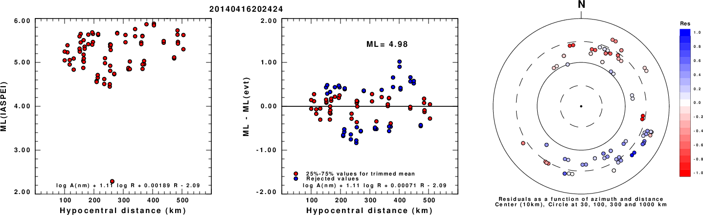
Left: ML computed using the IASPEI formula for Horizontal components. Center: ML residuals computed using a modified IASPEI formula that accounts for path specific attenuation; the values used for the trimmed mean are indicated. The ML relation used for each figure is given at the bottom of each plot.
Right: Residuals from new relation as a function of distance and azimuth.
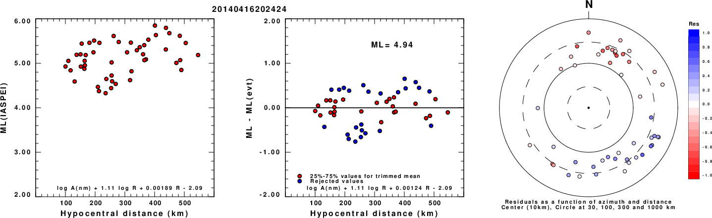
Left: ML computed using the IASPEI formula for Vertical components (research). Center: ML residuals computed using a modified IASPEI formula that accounts for path specific attenuation; the values used for the trimmed mean are indicated. The ML relation used for each figure is given at the bottom of each plot.
Right: Residuals from new relation as a function of distance and azimuth.
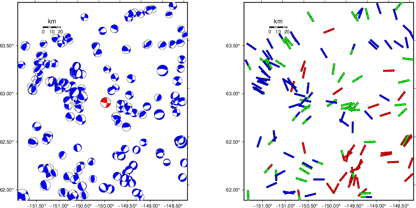
Context
The left panel of the next figure presents the focal mechanism for this earthquake (red) in the context of other nearby events (blue) in the SLU Moment Tensor Catalog. The right panel shows the inferred direction of maximum compressive stress and the type of faulting (green is strike-slip, red is normal, blue is thrust; oblique is shown by a combination of colors). Thus context plot is useful for assessing the appropriateness of the moment tensor of this event.
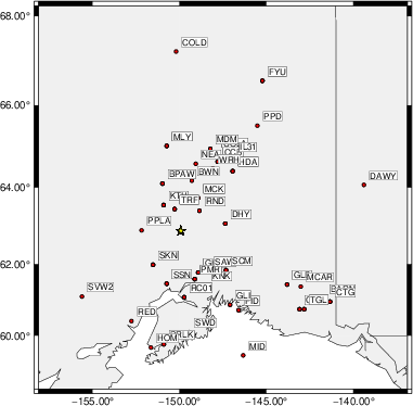
Waveform Inversion using wvfgrd96
The focal mechanism was determined using broadband seismic waveforms. The location of the event (star) and the
stations used for (red) the waveform inversion are shown in the next figure.
|
|
Location of broadband stations used for waveform inversion
|
The program wvfgrd96 was used with good traces observed at short distance to determine the focal mechanism, depth and seismic moment. This technique requires a high quality signal and well determined velocity model for the Green's functions. To the extent that these are the quality data, this type of mechanism should be preferred over the radiation pattern technique which requires the separate step of defining the pressure and tension quadrants and the correct strike.
The observed and predicted traces are filtered using the following gsac commands:
cut a -30 a 180
rtr
taper w 0.1
hp c 0.02 n 3
lp c 0.06 n 3
The results of this grid search are as follow:
           DEPTH  STK   DIP  RAKE   MW    FIT
WVFGRD96    2.0     5    85   -20   4.11 0.2424
WVFGRD96    4.0   185    90    15   4.19 0.2761
WVFGRD96    6.0     5    85   -10   4.24 0.2867
WVFGRD96    8.0   185    90    20   4.30 0.2922
WVFGRD96   10.0     5    80   -25   4.33 0.2983
WVFGRD96   12.0     5    80   -25   4.36 0.3012
WVFGRD96   14.0     5    85   -25   4.37 0.3017
WVFGRD96   16.0    95    85    20   4.37 0.3066
WVFGRD96   18.0   275    90   -20   4.39 0.3157
WVFGRD96   20.0    95    85    20   4.41 0.3276
WVFGRD96   22.0    95    85    20   4.44 0.3405
WVFGRD96   24.0    95    85    20   4.46 0.3531
WVFGRD96   26.0    95    85    15   4.48 0.3645
WVFGRD96   28.0    95    85    15   4.50 0.3753
WVFGRD96   30.0   100    80    15   4.53 0.3838
WVFGRD96   32.0   100    80    20   4.54 0.3924
WVFGRD96   34.0   100    80    20   4.56 0.4021
WVFGRD96   36.0   100    75    15   4.60 0.4112
WVFGRD96   38.0   100    75    15   4.63 0.4218
WVFGRD96   40.0   100    70    20   4.70 0.4371
WVFGRD96   42.0   100    70    20   4.72 0.4497
WVFGRD96   44.0   100    70    20   4.74 0.4621
WVFGRD96   46.0   100    70    20   4.76 0.4743
WVFGRD96   48.0   100    70    15   4.78 0.4874
WVFGRD96   50.0   100    70    15   4.80 0.5015
WVFGRD96   52.0   100    70    15   4.81 0.5163
WVFGRD96   54.0   100    75    20   4.82 0.5332
WVFGRD96   56.0   100    75    20   4.83 0.5504
WVFGRD96   58.0   100    75    20   4.85 0.5680
WVFGRD96   60.0   100    75    20   4.86 0.5861
WVFGRD96   62.0   100    75    20   4.87 0.6026
WVFGRD96   64.0   100    75    20   4.88 0.6179
WVFGRD96   66.0   100    75    20   4.89 0.6314
WVFGRD96   68.0   105    75    25   4.90 0.6442
WVFGRD96   70.0   105    75    25   4.91 0.6562
WVFGRD96   72.0   105    75    25   4.92 0.6661
WVFGRD96   74.0   105    75    25   4.93 0.6744
WVFGRD96   76.0   105    75    25   4.94 0.6810
WVFGRD96   78.0   100    80    25   4.93 0.6857
WVFGRD96   80.0   100    80    25   4.94 0.6892
WVFGRD96   82.0   100    80    25   4.94 0.6916
WVFGRD96   84.0   100    80    25   4.95 0.6922
WVFGRD96   86.0   100    85    25   4.94 0.6932
WVFGRD96   88.0   100    85    25   4.95 0.6929
WVFGRD96   90.0   100    85    25   4.95 0.6915
WVFGRD96   92.0   100    85    25   4.96 0.6888
WVFGRD96   94.0   100    85    25   4.96 0.6855
WVFGRD96   96.0   280    90   -25   4.95 0.6736
WVFGRD96   98.0   280    90   -25   4.96 0.6703
WVFGRD96  100.0   280    90   -25   4.96 0.6666
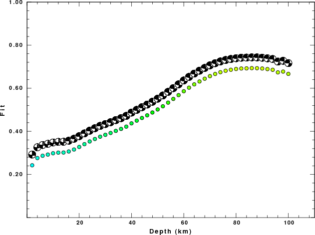
The best solution is
WVFGRD96 86.0 100 85 25 4.94 0.6932
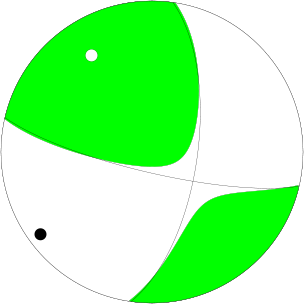
The mechanism corresponding to the best fit is
|
|
Figure 1. Waveform inversion focal mechanism
|
The best fit as a function of depth is given in the following figure:
|
|
Figure 2. Depth sensitivity for waveform mechanism
|
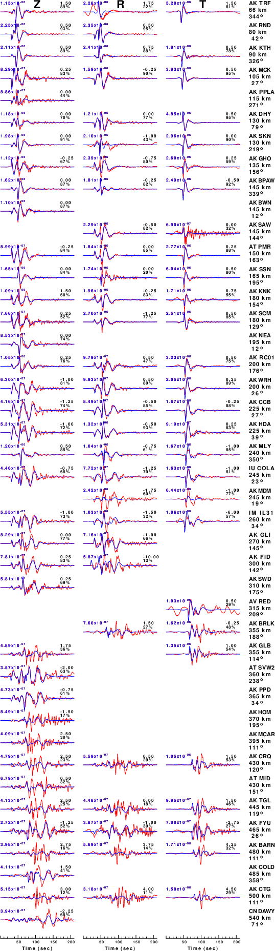
The comparison of the observed and predicted waveforms is given in the next figure. The red traces are the observed and the blue are the predicted.
Each observed-predicted component is plotted to the same scale and peak amplitudes are indicated by the numbers to the left of each trace. A pair of numbers is given in black at the right of each predicted traces. The upper number it the time shift required for maximum correlation between the observed and predicted traces. This time shift is required because the synthetics are not computed at exactly the same distance as the observed, the velocity model used in the predictions may not be perfect and the epicentral parameters may be be off.
A positive time shift indicates that the prediction is too fast and should be delayed to match the observed trace (shift to the right in this figure). A negative value indicates that the prediction is too slow. The lower number gives the percentage of variance reduction to characterize the individual goodness of fit (100% indicates a perfect fit).
The bandpass filter used in the processing and for the display was
cut a -30 a 180
rtr
taper w 0.1
hp c 0.02 n 3
lp c 0.06 n 3
|
|
Figure 3. Waveform comparison for selected depth. Red: observed; Blue - predicted. The time shift with respect to the model prediction is indicated. The percent of fit is also indicated. The time scale is relative to the first trace sample.
|
|
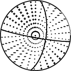
|
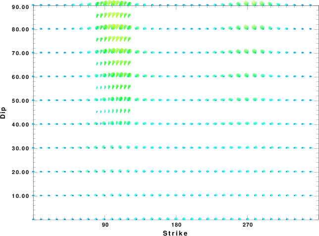
Focal mechanism sensitivity at the preferred depth. The red color indicates a very good fit to the waveforms.
Each solution is plotted as a vector at a given value of strike and dip with the angle of the vector representing the rake angle, measured, with respect to the upward vertical (N) in the figure.
|
A check on the assumed source location is possible by looking at the time shifts between the observed and predicted traces. The time shifts for waveform matching arise for several reasons:
- The origin time and epicentral distance are incorrect
- The velocity model used for the inversion is incorrect
- The velocity model used to define the P-arrival time is not the
same as the velocity model used for the waveform inversion
(assuming that the initial trace alignment is based on the
P arrival time)
Assuming only a mislocation, the time shifts are fit to a functional form:
Time_shift = A + B cos Azimuth + C Sin Azimuth
The time shifts for this inversion lead to the next figure:
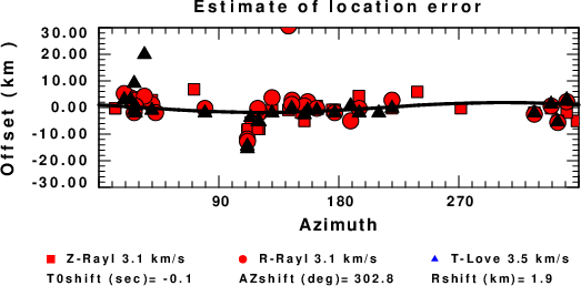
The derived shift in origin time and epicentral coordinates are given at the bottom of the figure.
Velocity Model
The WUS.model used for the waveform synthetic seismograms and for the surface wave eigenfunctions and dispersion is as follows
(The format is in the model96 format of Computer Programs in Seismology).
MODEL.01
Model after     8 iterations
ISOTROPIC
KGS
FLAT EARTH
1-D
CONSTANT VELOCITY
LINE08
LINE09
LINE10
LINE11
      H(KM)   VP(KM/S)   VS(KM/S) RHO(GM/CC)         QP         QS       ETAP       ETAS      FREFP      FREFS
     1.9000     3.4065     2.0089     2.2150  0.302E-02  0.679E-02   0.00       0.00       1.00       1.00
     6.1000     5.5445     3.2953     2.6089  0.349E-02  0.784E-02   0.00       0.00       1.00       1.00
    13.0000     6.2708     3.7396     2.7812  0.212E-02  0.476E-02   0.00       0.00       1.00       1.00
    19.0000     6.4075     3.7680     2.8223  0.111E-02  0.249E-02   0.00       0.00       1.00       1.00
     0.0000     7.9000     4.6200     3.2760  0.164E-10  0.370E-10   0.00       0.00       1.00       1.00
Last Changed Fri Apr 26 05:45:01 PM CDT 2024