Location
Location ANSS
The ANSS event ID is usb000pkhs and the event page is at
https://earthquake.usgs.gov/earthquakes/eventpage/usb000pkhs/executive.
2014/04/14 20:16:47 44.600 -114.330 7.4 4.4 Idaho
Focal Mechanism
 USGS/SLU Moment Tensor Solution
 ENS  2014/04/14 20:16:47:0  44.60 -114.33   7.4 4.4 Idaho

 Stations used:
   CN.WALA IM.PD31 IW.DLMT IW.FLWY IW.FXWY IW.IMW IW.MFID
   IW.REDW IW.SNOW IW.TPAW MB.JTMT TA.H17A UO.PINE US.AHID
   US.BMO US.BW06 US.DUG US.EGMT US.ELK US.HAWA US.HWUT
   US.LKWY US.MSO US.NEW US.RLMT UU.BGU UU.CTU UU.HVU UU.JLU
   UU.MPU UU.NLU UU.RDMU UU.SPU UU.TCU UW.CCRK UW.DAVN UW.DDRF
   UW.IRON UW.IZEE UW.LTY UW.OMAK UW.PHIN UW.TREE UW.TUCA
   UW.UMAT UW.WOLL WY.YHB WY.YHH WY.YHL WY.YMP WY.YMR WY.YNM
   WY.YNR WY.YPP WY.YUF

 Filtering commands used:
   cut o DIST/3.3 -40 o DIST/3.3 +50
   rtr
   taper w 0.1
   hp c 0.03 n 3
   lp c 0.07 n 3

 Best Fitting Double Couple
  Mo = 3.55e+22 dyne-cm
  Mw = 4.30
  Z  = 12 km
  Plane   Strike  Dip  Rake
   NP1       92    71   -159
   NP2      355    70   -20
  Principal Axes:
   Axis    Value   Plunge  Azimuth
    T   3.55e+22      1     223
    N   0.00e+00     62     132
    P  -3.55e+22     28     314

 Moment Tensor: (dyne-cm)
    Component   Value
       Mxx     5.50e+21
       Mxy     3.15e+22
       Mxz    -1.05e+22
       Myy     2.30e+21
       Myz     1.03e+22
       Mzz    -7.80e+21


                     ------########
                 -----------###########
              ---------------#############
             -----------------#############
           -----   ------------##############
          ------ P ------------###############
         -------   -------------###############
        ------------------------################
        -------------------------###############
       --------------------------################
       --------------------------################
       ###-----------------------###############-
       ########------------------###########-----
        #################--------##-------------
        #########################---------------
         ########################--------------
          #######################-------------
           ######################------------
                ################-----------
              T ################----------
                 ##############--------
                     #########-----


 Global CMT Convention Moment Tensor:
      R          T          P
 -7.80e+21  -1.05e+22  -1.03e+22
 -1.05e+22   5.50e+21  -3.15e+22
 -1.03e+22  -3.15e+22   2.30e+21


Details of the solution is found at

http://www.eas.slu.edu/eqc/eqc_mt/MECH.NA/20140414201647/index.html
|
Preferred Solution
The preferred solution from an analysis of the surface-wave spectral amplitude radiation pattern, waveform inversion or first motion observations is
      STK = -5
      DIP = 70
     RAKE = -20
       MW = 4.30
       HS = 12.0
The NDK file is 20140414201647.ndk
The waveform inversion is preferred.
Moment Tensor Comparison
The following compares this source inversion to those provided by others. The purpose is to look for major differences and also to note slight differences that might be inherent to the processing procedure. For completeness the USGS/SLU solution is repeated from above.
| SLU |
USGSMT |
 USGS/SLU Moment Tensor Solution
 ENS  2014/04/14 20:16:47:0  44.60 -114.33   7.4 4.4 Idaho

 Stations used:
   CN.WALA IM.PD31 IW.DLMT IW.FLWY IW.FXWY IW.IMW IW.MFID
   IW.REDW IW.SNOW IW.TPAW MB.JTMT TA.H17A UO.PINE US.AHID
   US.BMO US.BW06 US.DUG US.EGMT US.ELK US.HAWA US.HWUT
   US.LKWY US.MSO US.NEW US.RLMT UU.BGU UU.CTU UU.HVU UU.JLU
   UU.MPU UU.NLU UU.RDMU UU.SPU UU.TCU UW.CCRK UW.DAVN UW.DDRF
   UW.IRON UW.IZEE UW.LTY UW.OMAK UW.PHIN UW.TREE UW.TUCA
   UW.UMAT UW.WOLL WY.YHB WY.YHH WY.YHL WY.YMP WY.YMR WY.YNM
   WY.YNR WY.YPP WY.YUF

 Filtering commands used:
   cut o DIST/3.3 -40 o DIST/3.3 +50
   rtr
   taper w 0.1
   hp c 0.03 n 3
   lp c 0.07 n 3

 Best Fitting Double Couple
  Mo = 3.55e+22 dyne-cm
  Mw = 4.30
  Z  = 12 km
  Plane   Strike  Dip  Rake
   NP1       92    71   -159
   NP2      355    70   -20
  Principal Axes:
   Axis    Value   Plunge  Azimuth
    T   3.55e+22      1     223
    N   0.00e+00     62     132
    P  -3.55e+22     28     314

 Moment Tensor: (dyne-cm)
    Component   Value
       Mxx     5.50e+21
       Mxy     3.15e+22
       Mxz    -1.05e+22
       Myy     2.30e+21
       Myz     1.03e+22
       Mzz    -7.80e+21


                     ------########
                 -----------###########
              ---------------#############
             -----------------#############
           -----   ------------##############
          ------ P ------------###############
         -------   -------------###############
        ------------------------################
        -------------------------###############
       --------------------------################
       --------------------------################
       ###-----------------------###############-
       ########------------------###########-----
        #################--------##-------------
        #########################---------------
         ########################--------------
          #######################-------------
           ######################------------
                ################-----------
              T ################----------
                 ##############--------
                     #########-----


 Global CMT Convention Moment Tensor:
      R          T          P
 -7.80e+21  -1.05e+22  -1.03e+22
 -1.05e+22   5.50e+21  -3.15e+22
 -1.03e+22  -3.15e+22   2.30e+21


Details of the solution is found at

http://www.eas.slu.edu/eqc/eqc_mt/MECH.NA/20140414201647/index.html
|
Regional Moment Tensor (Mwr)

Moment magnitude derived from a moment tensor
inversion of complete waveforms at regional
distances (less than ~8 degrees), generally
used for the analysis of small to moderate
size earthquakes (typically Mw 3.5-6.0)
crust or upper mantle earthquakes.

Moment
4.75e+15 N-m
Magnitude
4.4
Percent DC
75%
Depth
8.0 km
Updated
2014-04-14 21:01:18 UTC
Author
us
Catalog
us
Contributor
us
Code
us_b000pkhs_mwr
Principal Axes

Axis	Value	Plunge	Azimuth
T	5.034	5	43
N	-0.623	8	312
P	-4.411	81	165
Nodal Planes

Plane	Strike	Dip	Rake
NP1	305	51	-100
NP2	142	41	-78
|
|
Magnitudes
Given the availability of digital waveforms for determination of the moment tensor, this section documents the added processing leading to mLg, if appropriate to the region, and ML by application of the respective IASPEI formulae. As a research study, the linear distance term of the IASPEI formula
for ML is adjusted to remove a linear distance trend in residuals to give a regionally defined ML. The defined ML uses horizontal component recordings, but the same procedure is applied to the vertical components since there may be some interest in vertical component ground motions. Residual plots versus distance may indicate interesting features of ground motion scaling in some distance ranges. A residual plot of the regionalized magnitude is given as a function of distance and azimuth, since data sets may transcend different wave propagation provinces.
ML Magnitude
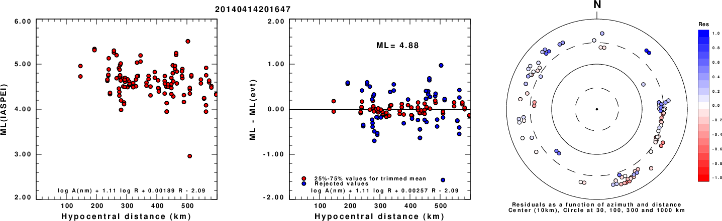
Left: ML computed using the IASPEI formula for Horizontal components. Center: ML residuals computed using a modified IASPEI formula that accounts for path specific attenuation; the values used for the trimmed mean are indicated. The ML relation used for each figure is given at the bottom of each plot.
Right: Residuals from new relation as a function of distance and azimuth.
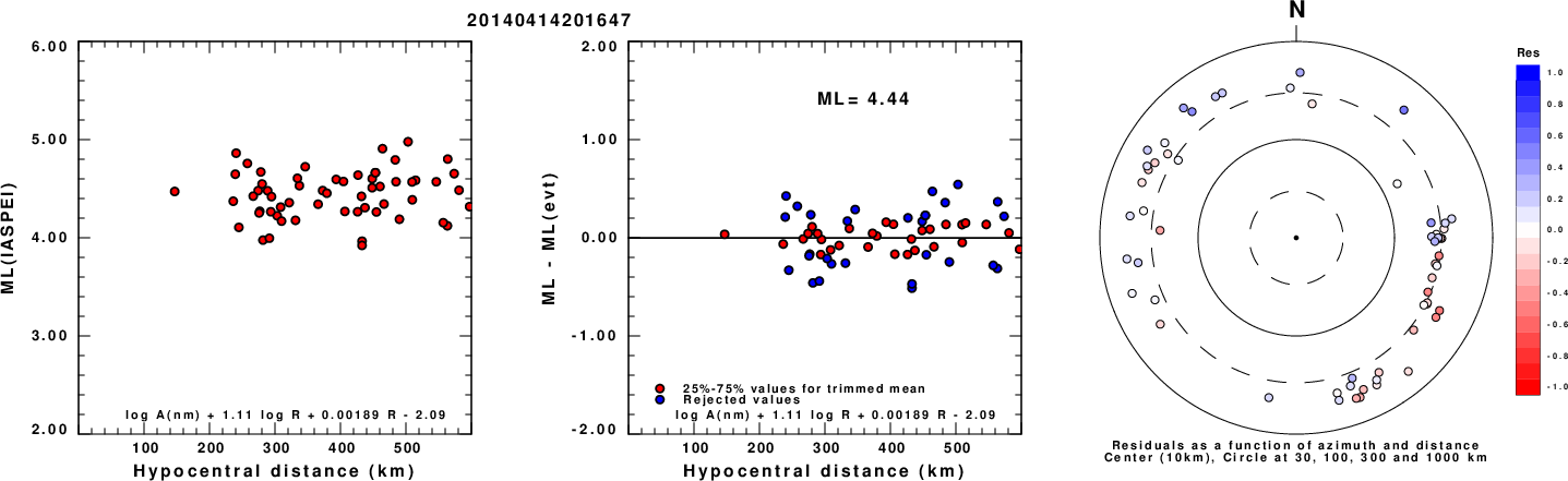
Left: ML computed using the IASPEI formula for Vertical components (research). Center: ML residuals computed using a modified IASPEI formula that accounts for path specific attenuation; the values used for the trimmed mean are indicated. The ML relation used for each figure is given at the bottom of each plot.
Right: Residuals from new relation as a function of distance and azimuth.
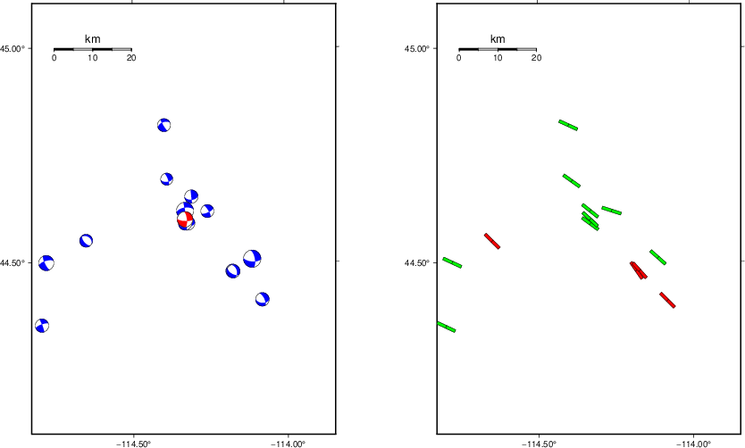
Context
The left panel of the next figure presents the focal mechanism for this earthquake (red) in the context of other nearby events (blue) in the SLU Moment Tensor Catalog. The right panel shows the inferred direction of maximum compressive stress and the type of faulting (green is strike-slip, red is normal, blue is thrust; oblique is shown by a combination of colors). Thus context plot is useful for assessing the appropriateness of the moment tensor of this event.
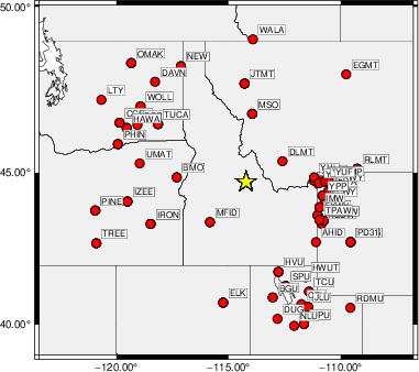
Waveform Inversion using wvfgrd96
The focal mechanism was determined using broadband seismic waveforms. The location of the event (star) and the
stations used for (red) the waveform inversion are shown in the next figure.
|
|
Location of broadband stations used for waveform inversion
|
The program wvfgrd96 was used with good traces observed at short distance to determine the focal mechanism, depth and seismic moment. This technique requires a high quality signal and well determined velocity model for the Green's functions. To the extent that these are the quality data, this type of mechanism should be preferred over the radiation pattern technique which requires the separate step of defining the pressure and tension quadrants and the correct strike.
The observed and predicted traces are filtered using the following gsac commands:
cut o DIST/3.3 -40 o DIST/3.3 +50
rtr
taper w 0.1
hp c 0.03 n 3
lp c 0.07 n 3
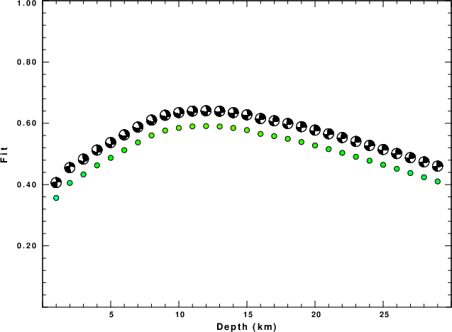
The results of this grid search are as follow:
           DEPTH  STK   DIP  RAKE   MW    FIT
WVFGRD96    1.0   355    80    10   3.98 0.3565
WVFGRD96    2.0    -5    90    25   4.07 0.4054
WVFGRD96    3.0   175    90    40   4.14 0.4332
WVFGRD96    4.0    -5    85   -40   4.17 0.4628
WVFGRD96    5.0   355    80   -35   4.17 0.4873
WVFGRD96    6.0   350    60   -30   4.21 0.5124
WVFGRD96    7.0   350    60   -30   4.23 0.5378
WVFGRD96    8.0   350    55   -35   4.28 0.5605
WVFGRD96    9.0   350    60   -30   4.28 0.5764
WVFGRD96   10.0   355    65   -25   4.28 0.5850
WVFGRD96   11.0   355    65   -25   4.30 0.5899
WVFGRD96   12.0    -5    70   -20   4.30 0.5909
WVFGRD96   13.0    -5    70   -20   4.31 0.5895
WVFGRD96   14.0    -5    70   -20   4.32 0.5848
WVFGRD96   15.0    -5    70   -15   4.33 0.5779
WVFGRD96   16.0   180    75    15   4.34 0.5655
WVFGRD96   17.0   180    75    15   4.35 0.5582
WVFGRD96   18.0   180    75    15   4.35 0.5492
WVFGRD96   19.0   180    75    15   4.36 0.5390
WVFGRD96   20.0   180    75    15   4.37 0.5278
WVFGRD96   21.0   180    75    15   4.38 0.5158
WVFGRD96   22.0   180    75    15   4.38 0.5035
WVFGRD96   23.0   180    75    15   4.39 0.4908
WVFGRD96   24.0   180    75    10   4.39 0.4779
WVFGRD96   25.0   180    75    10   4.40 0.4647
WVFGRD96   26.0   180    75    10   4.40 0.4514
WVFGRD96   27.0   180    75    10   4.41 0.4378
WVFGRD96   28.0   180    75    10   4.41 0.4241
WVFGRD96   29.0   180    75    10   4.42 0.4104
The best solution is
WVFGRD96 12.0 -5 70 -20 4.30 0.5909
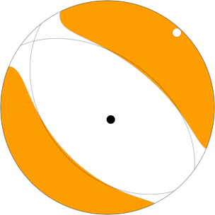
The mechanism corresponding to the best fit is
|
|
Figure 1. Waveform inversion focal mechanism
|
The best fit as a function of depth is given in the following figure:
|
|
Figure 2. Depth sensitivity for waveform mechanism
|
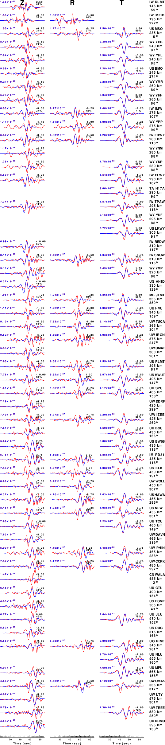
The comparison of the observed and predicted waveforms is given in the next figure. The red traces are the observed and the blue are the predicted.
Each observed-predicted component is plotted to the same scale and peak amplitudes are indicated by the numbers to the left of each trace. A pair of numbers is given in black at the right of each predicted traces. The upper number it the time shift required for maximum correlation between the observed and predicted traces. This time shift is required because the synthetics are not computed at exactly the same distance as the observed, the velocity model used in the predictions may not be perfect and the epicentral parameters may be be off.
A positive time shift indicates that the prediction is too fast and should be delayed to match the observed trace (shift to the right in this figure). A negative value indicates that the prediction is too slow. The lower number gives the percentage of variance reduction to characterize the individual goodness of fit (100% indicates a perfect fit).
The bandpass filter used in the processing and for the display was
cut o DIST/3.3 -40 o DIST/3.3 +50
rtr
taper w 0.1
hp c 0.03 n 3
lp c 0.07 n 3
|
|
Figure 3. Waveform comparison for selected depth. Red: observed; Blue - predicted. The time shift with respect to the model prediction is indicated. The percent of fit is also indicated. The time scale is relative to the first trace sample.
|
|
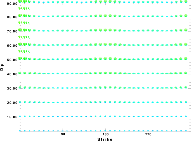
|
Focal mechanism sensitivity at the preferred depth. The red color indicates a very good fit to the waveforms.
Each solution is plotted as a vector at a given value of strike and dip with the angle of the vector representing the rake angle, measured, with respect to the upward vertical (N) in the figure.
|
A check on the assumed source location is possible by looking at the time shifts between the observed and predicted traces. The time shifts for waveform matching arise for several reasons:
- The origin time and epicentral distance are incorrect
- The velocity model used for the inversion is incorrect
- The velocity model used to define the P-arrival time is not the
same as the velocity model used for the waveform inversion
(assuming that the initial trace alignment is based on the
P arrival time)
Assuming only a mislocation, the time shifts are fit to a functional form:
Time_shift = A + B cos Azimuth + C Sin Azimuth
The time shifts for this inversion lead to the next figure:
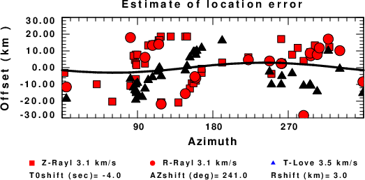
The derived shift in origin time and epicentral coordinates are given at the bottom of the figure.
Surface-Wave Focal Mechanism
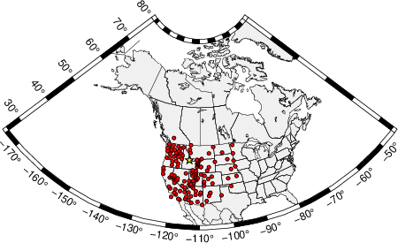
The following figure shows the stations used in the grid search for the best focal mechanism to fit the surface-wave spectral amplitudes of the Love and Rayleigh waves.
|
|
Location of broadband stations used to obtain focal mechanism from surface-wave spectral amplitudes
|
The surface-wave determined focal mechanism is shown here.
  NODAL PLANES


  STK=     289.99
  DIP=      55.00
 RAKE=    -125.00

             OR

  STK=     160.66
  DIP=      47.85
 RAKE=     -50.68


DEPTH = 8.0 km

Mw = 4.42
Best Fit 0.9011 - P-T axis plot gives solutions with FIT greater than FIT90
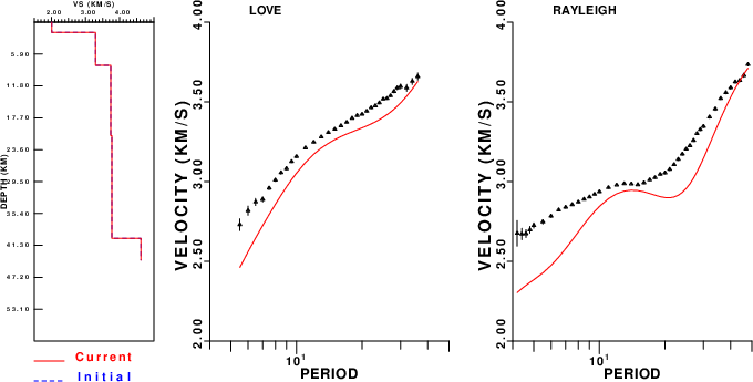
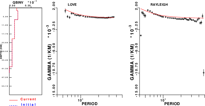
Surface-wave analysis
Surface wave analysis was performed using codes from
Computer Programs in Seismology, specifically the
multiple filter analysis program do_mft and the surface-wave
radiation pattern search program srfgrd96.
Data preparation
Digital data were collected, instrument response removed and traces converted
to Z, R an T components. Multiple filter analysis was applied to the Z and T traces to obtain the Rayleigh- and Love-wave spectral amplitudes, respectively.
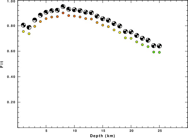
These were input to the search program which examined all depths between 1 and 25 km
and all possible mechanisms.
|
|
Best mechanism fit as a function of depth. The preferred depth is given above. Lower hemisphere projection
|
|
|
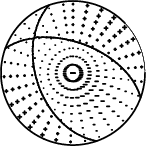
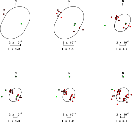
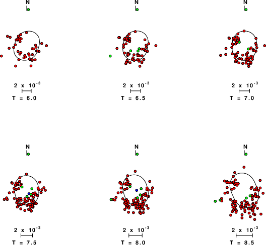
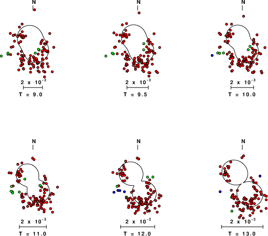
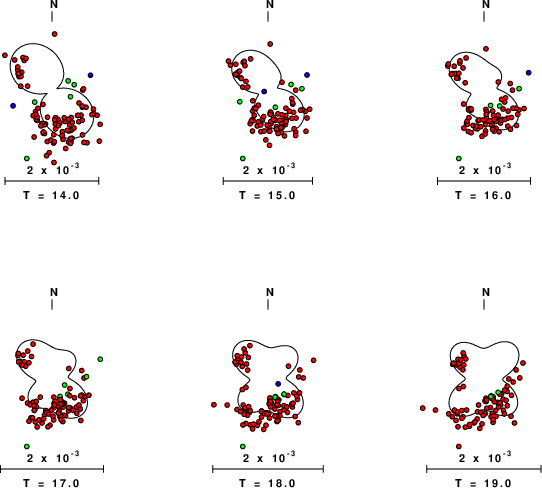
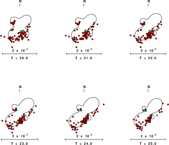
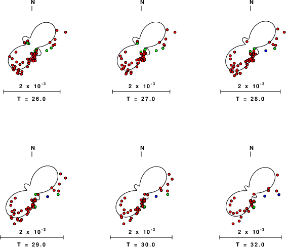
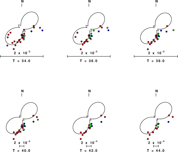
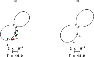
Pressure-tension axis trends. Since the surface-wave spectra search does not distinguish between P and T axes and since there is a 180 ambiguity in strike, all possible P and T axes are plotted. First motion data and waveforms will be used to select the preferred mechanism. The purpose of this plot is to provide an idea of the
possible range of solutions. The P and T-axes for all mechanisms with goodness of fit greater than 0.9 FITMAX (above) are plotted here.
|
|
|
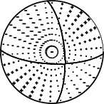
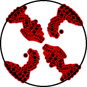
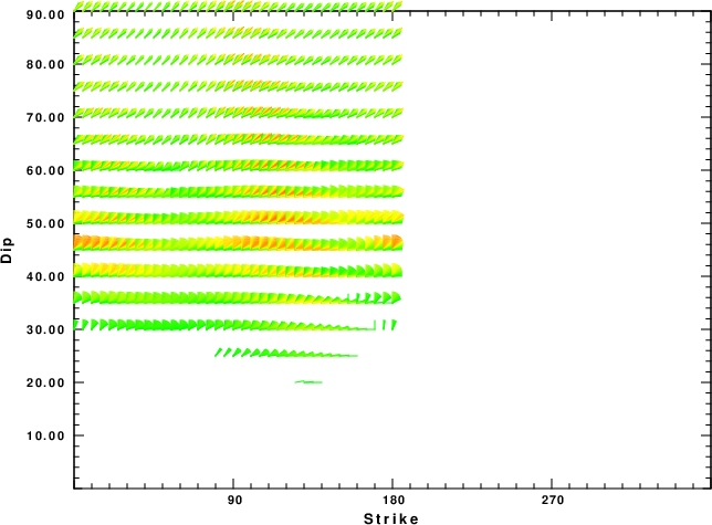
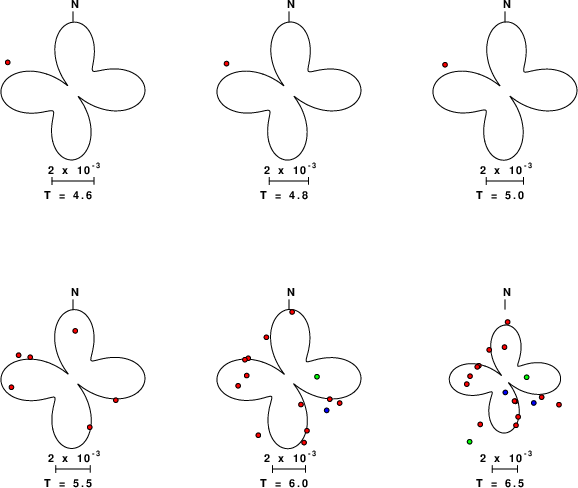
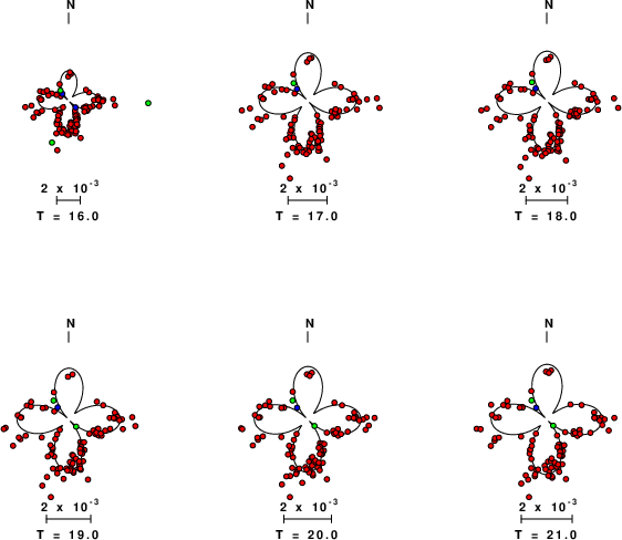
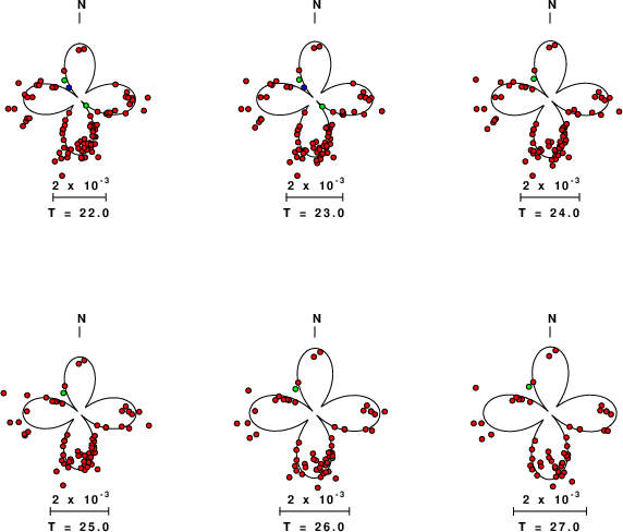
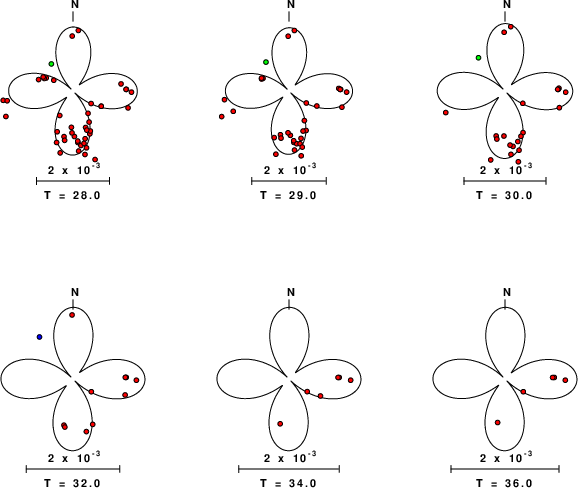
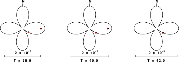
Focal mechanism sensitivity at the preferred depth. The red color indicates a very good fit to the Love and Rayleigh wave radiation patterns.
Each solution is plotted as a vector at a given value of strike and dip with the angle of the vector representing the rake angle, measured, with respect to the upward vertical (N) in the figure. Because of the symmetry of the spectral amplitude rediation patterns, only strikes from 0-180 degrees are sampled.
|
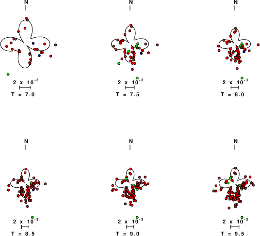
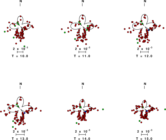
Love-wave radiation patterns
Rayleigh-wave radiation patterns