Location

Location ANSS

The ANSS event ID is usc000nxm5 and the event page is at https://earthquake.usgs.gov/earthquakes/eventpage/usc000nxm5/executive.

2014/03/31 16:30:27 62.288 -124.522 1.0 4.3 NT, Canada

Focal Mechanism

USGS/SLU Moment Tensor Solution ENS 2014/03/31 16:30:27:0 62.29 -124.52 1.0 4.3 NT, Canada Stations used: AK.BESE AT.SIT AT.SKAG CN.DHRN CN.DLBC CN.EDZN CN.HYT CN.INK CN.WHY CN.YKW3 CN.YUK1 CN.YUK2 CN.YUK3 CN.YUK4 CN.YUK6 TA.C36M TA.EPYK US.EGAK US.WRAK Filtering commands used: cut o DIST/3.2 -100 o DIST/3.2 +80 rtr taper w 0.1 hp c 0.02 n 3 lp c 0.06 n 3 Best Fitting Double Couple Mo = 2.69e+22 dyne-cm Mw = 4.22 Z = 6 km Plane Strike Dip Rake NP1 310 55 75 NP2 155 38 110 Principal Axes: Axis Value Plunge Azimuth T 2.69e+22 75 176 N 0.00e+00 12 319 P -2.69e+22 9 51 Moment Tensor: (dyne-cm) Component Value Mxx -8.72e+21 Mxy -1.30e+22 Mxz -9.38e+21 Myy -1.57e+22 Myz -2.65e+21 Mzz 2.44e+22 -------------- #--------------------- ###------------------------- ###------------------------- ----##########---------------- P - -----##############------------ -- -----##################--------------- ------####################-------------- ------######################------------ -------########################----------- -------#########################---------- --------#########################--------- --------############ ###########-------- --------########### T ############------ ---------########## #############----- ---------##########################--- ---------#########################-- ----------#######################- ----------#################### -----------################# ------------########## -------------- Global CMT Convention Moment Tensor: R T P 2.44e+22 -9.38e+21 2.65e+21 -9.38e+21 -8.72e+21 1.30e+22 2.65e+21 1.30e+22 -1.57e+22 Details of the solution is found at http://www.eas.slu.edu/eqc/eqc_mt/MECH.NA/20140331163027/index.html

Preferred Solution

The preferred solution from an analysis of the surface-wave spectral amplitude radiation pattern, waveform inversion or first motion observations is

      STK = 310
      DIP = 55
     RAKE = 75
       MW = 4.22
       HS = 6.0

The NDK file is 20140331163027.ndk The waveform inversion is preferred.

Context

The left panel of the next figure presents the focal mechanism for this earthquake (red) in the context of other nearby events (blue) in the SLU Moment Tensor Catalog. The right panel shows the inferred direction of maximum compressive stress and the type of faulting (green is strike-slip, red is normal, blue is thrust; oblique is shown by a combination of colors). Thus context plot is useful for assessing the appropriateness of the moment tensor of this event.

Waveform Inversion using wvfgrd96

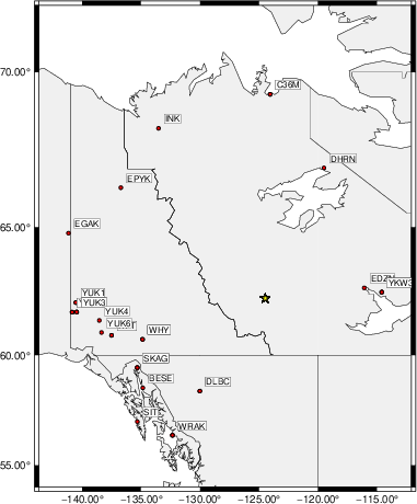
The focal mechanism was determined using broadband seismic waveforms. The location of the event (star) and the stations used for (red) the waveform inversion are shown in the next figure.

Location of broadband stations used for waveform inversion

The program wvfgrd96 was used with good traces observed at short distance to determine the focal mechanism, depth and seismic moment. This technique requires a high quality signal and well determined velocity model for the Green's functions. To the extent that these are the quality data, this type of mechanism should be preferred over the radiation pattern technique which requires the separate step of defining the pressure and tension quadrants and the correct strike.

The observed and predicted traces are filtered using the following gsac commands:

cut o DIST/3.2 -100 o DIST/3.2 +80
rtr
taper w 0.1
hp c 0.02 n 3 
lp c 0.06 n 3

The results of this grid search are as follow:

           DEPTH  STK   DIP  RAKE   MW    FIT
WVFGRD96    1.0   100    90   -60   4.20 0.5838
WVFGRD96    2.0   285    80    45   4.10 0.6122
WVFGRD96    3.0   285    80    45   4.13 0.6247
WVFGRD96    4.0   295    65    60   4.17 0.6250
WVFGRD96    5.0   310    55    75   4.21 0.6601
WVFGRD96    6.0   310    55    75   4.22 0.6619
WVFGRD96    7.0   300    60    60   4.19 0.6339
WVFGRD96    8.0   100    80   -20   4.11 0.6165
WVFGRD96    9.0   100    80   -20   4.12 0.6132
WVFGRD96   10.0   275    65   -20   4.12 0.6207
WVFGRD96   11.0   275    65   -20   4.13 0.6232
WVFGRD96   12.0   275    65   -15   4.13 0.6246
WVFGRD96   13.0   275    65   -15   4.13 0.6251
WVFGRD96   14.0   275    65   -15   4.14 0.6246
WVFGRD96   15.0   275    65   -15   4.14 0.6231
WVFGRD96   16.0   275    65   -15   4.15 0.6207
WVFGRD96   17.0   275    65   -15   4.16 0.6176
WVFGRD96   18.0   275    65   -15   4.16 0.6139
WVFGRD96   19.0   275    65   -15   4.17 0.6095
WVFGRD96   20.0   275    65   -15   4.19 0.6069
WVFGRD96   21.0   275    65   -15   4.19 0.6019
WVFGRD96   22.0   275    65   -15   4.20 0.5964
WVFGRD96   23.0   275    65   -15   4.21 0.5905
WVFGRD96   24.0   275    65   -15   4.21 0.5843
WVFGRD96   25.0   275    65   -15   4.22 0.5779
WVFGRD96   26.0   275    65   -15   4.23 0.5711
WVFGRD96   27.0   275    65   -15   4.23 0.5641
WVFGRD96   28.0   275    65   -20   4.24 0.5574
WVFGRD96   29.0   275    65   -20   4.25 0.5506

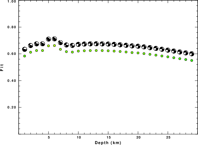
The best solution is

WVFGRD96    6.0   310    55    75   4.22 0.6619

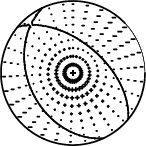
The mechanism corresponding to the best fit is

Figure 1. Waveform inversion focal mechanism

The best fit as a function of depth is given in the following figure:

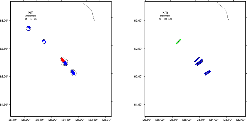
Figure 2. Depth sensitivity for waveform mechanism

The comparison of the observed and predicted waveforms is given in the next figure. The red traces are the observed and the blue are the predicted. Each observed-predicted component is plotted to the same scale and peak amplitudes are indicated by the numbers to the left of each trace. A pair of numbers is given in black at the right of each predicted traces. The upper number it the time shift required for maximum correlation between the observed and predicted traces. This time shift is required because the synthetics are not computed at exactly the same distance as the observed, the velocity model used in the predictions may not be perfect and the epicentral parameters may be be off. A positive time shift indicates that the prediction is too fast and should be delayed to match the observed trace (shift to the right in this figure). A negative value indicates that the prediction is too slow. The lower number gives the percentage of variance reduction to characterize the individual goodness of fit (100% indicates a perfect fit).

The bandpass filter used in the processing and for the display was

cut o DIST/3.2 -100 o DIST/3.2 +80
rtr
taper w 0.1
hp c 0.02 n 3 
lp c 0.06 n 3

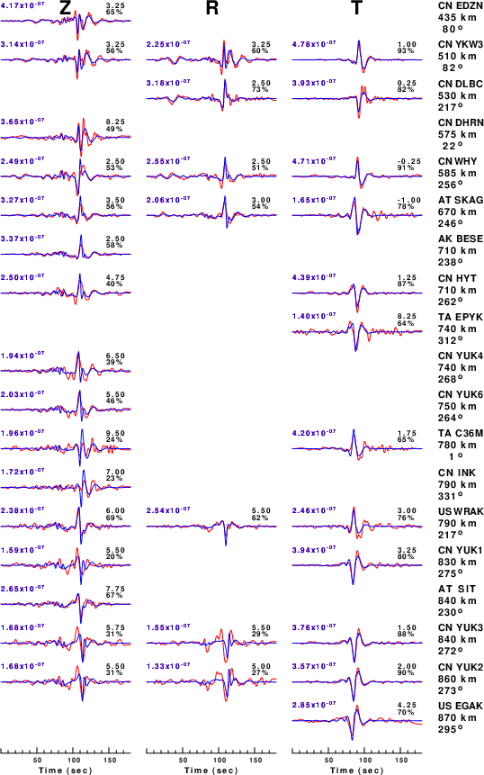
Figure 3. Waveform comparison for selected depth. Red: observed; Blue - predicted. The time shift with respect to the model prediction is indicated. The percent of fit is also indicated. The time scale is relative to the first trace sample.

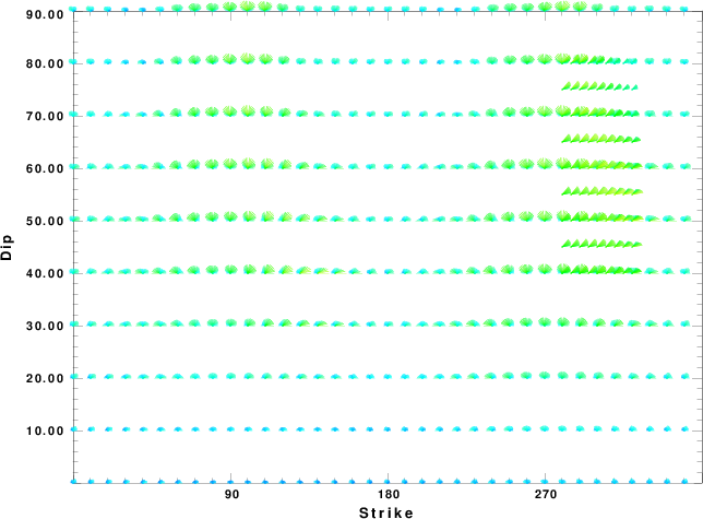
Focal mechanism sensitivity at the preferred depth. The red color indicates a very good fit to the waveforms. Each solution is plotted as a vector at a given value of strike and dip with the angle of the vector representing the rake angle, measured, with respect to the upward vertical (N) in the figure.

A check on the assumed source location is possible by looking at the time shifts between the observed and predicted traces. The time shifts for waveform matching arise for several reasons:

The origin time and epicentral distance are incorrect
The velocity model used for the inversion is incorrect
The velocity model used to define the P-arrival time is not the same as the velocity model used for the waveform inversion (assuming that the initial trace alignment is based on the P arrival time)

Assuming only a mislocation, the time shifts are fit to a functional form:

 Time_shift = A + B cos Azimuth + C Sin Azimuth

The time shifts for this inversion lead to the next figure:

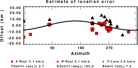
The derived shift in origin time and epicentral coordinates are given at the bottom of the figure.

Velocity Model

The WUS.model used for the waveform synthetic seismograms and for the surface wave eigenfunctions and dispersion is as follows (The format is in the model96 format of Computer Programs in Seismology).

MODEL.01
Model after     8 iterations
ISOTROPIC
KGS
FLAT EARTH
1-D
CONSTANT VELOCITY
LINE08
LINE09
LINE10
LINE11
      H(KM)   VP(KM/S)   VS(KM/S) RHO(GM/CC)         QP         QS       ETAP       ETAS      FREFP      FREFS
     1.9000     3.4065     2.0089     2.2150  0.302E-02  0.679E-02   0.00       0.00       1.00       1.00    
     6.1000     5.5445     3.2953     2.6089  0.349E-02  0.784E-02   0.00       0.00       1.00       1.00    
    13.0000     6.2708     3.7396     2.7812  0.212E-02  0.476E-02   0.00       0.00       1.00       1.00    
    19.0000     6.4075     3.7680     2.8223  0.111E-02  0.249E-02   0.00       0.00       1.00       1.00    
     0.0000     7.9000     4.6200     3.2760  0.164E-10  0.370E-10   0.00       0.00       1.00       1.00

Last Changed Sat Apr 27 10:40:43 AM CDT 2024