Location
Location ANSS
The ANSS event ID is ak01439k6eg1 and the event page is at
https://earthquake.usgs.gov/earthquakes/eventpage/ak01439k6eg1/executive.
2014/03/12 08:43:35 59.288 -153.169 85.9 4.6 Alaska
Focal Mechanism
 USGS/SLU Moment Tensor Solution
 ENS  2014/03/12 08:43:35:0  59.29 -153.17  85.9 4.6 Alaska

 Stations used:
   AK.BRLK AK.CNP AK.GHO AK.HOM AK.KNK AK.KTH AK.RC01 AK.SAW
   AK.SCM AK.SII AK.SWD AT.OHAK AT.PMR AT.SVW2

 Filtering commands used:
   cut a -30 a 180
   rtr
   taper w 0.1
   hp c 0.02 n 3
   lp c 0.06 n 3

 Best Fitting Double Couple
  Mo = 1.32e+23 dyne-cm
  Mw = 4.68
  Z  = 85 km
  Plane   Strike  Dip  Rake
   NP1       65    75    45
   NP2      320    47   159
  Principal Axes:
   Axis    Value   Plunge  Azimuth
    T   1.32e+23     42     293
    N   0.00e+00     43      80
    P  -1.32e+23     17     187

 Moment Tensor: (dyne-cm)
    Component   Value
       Mxx    -1.07e+23
       Mxy    -4.00e+22
       Mxz     6.30e+22
       Myy     6.06e+22
       Myz    -5.60e+22
       Mzz     4.66e+22


                     --------------
                 ----------------------
              #########-------------------
             ###############---------------
           ####################--------------
          #######################-------------
         ##########################-----------#
        #######   ###################--------###
        ####### T ####################-----#####
       ########   #####################-#########
       ###############################--#########
       ############################------########
       ########################-----------#######
        ###################---------------######
        ##############--------------------######
         ######---------------------------#####
          --------------------------------####
           -------------------------------###
             -----------------------------#
              -----------   -------------#
                 -------- P -----------
                     ----   -------


 Global CMT Convention Moment Tensor:
      R          T          P
  4.66e+22   6.30e+22   5.60e+22
  6.30e+22  -1.07e+23   4.00e+22
  5.60e+22   4.00e+22   6.06e+22


Details of the solution is found at

http://www.eas.slu.edu/eqc/eqc_mt/MECH.NA/20140312084335/index.html
|
Preferred Solution
The preferred solution from an analysis of the surface-wave spectral amplitude radiation pattern, waveform inversion or first motion observations is
      STK = 65
      DIP = 75
     RAKE = 45
       MW = 4.68
       HS = 85.0
The NDK file is 20140312084335.ndk
The waveform inversion is preferred.
Moment Tensor Comparison
The following compares this source inversion to those provided by others. The purpose is to look for major differences and also to note slight differences that might be inherent to the processing procedure. For completeness the USGS/SLU solution is repeated from above.
| SLU |
USGSMT |
 USGS/SLU Moment Tensor Solution
 ENS  2014/03/12 08:43:35:0  59.29 -153.17  85.9 4.6 Alaska

 Stations used:
   AK.BRLK AK.CNP AK.GHO AK.HOM AK.KNK AK.KTH AK.RC01 AK.SAW
   AK.SCM AK.SII AK.SWD AT.OHAK AT.PMR AT.SVW2

 Filtering commands used:
   cut a -30 a 180
   rtr
   taper w 0.1
   hp c 0.02 n 3
   lp c 0.06 n 3

 Best Fitting Double Couple
  Mo = 1.32e+23 dyne-cm
  Mw = 4.68
  Z  = 85 km
  Plane   Strike  Dip  Rake
   NP1       65    75    45
   NP2      320    47   159
  Principal Axes:
   Axis    Value   Plunge  Azimuth
    T   1.32e+23     42     293
    N   0.00e+00     43      80
    P  -1.32e+23     17     187

 Moment Tensor: (dyne-cm)
    Component   Value
       Mxx    -1.07e+23
       Mxy    -4.00e+22
       Mxz     6.30e+22
       Myy     6.06e+22
       Myz    -5.60e+22
       Mzz     4.66e+22


                     --------------
                 ----------------------
              #########-------------------
             ###############---------------
           ####################--------------
          #######################-------------
         ##########################-----------#
        #######   ###################--------###
        ####### T ####################-----#####
       ########   #####################-#########
       ###############################--#########
       ############################------########
       ########################-----------#######
        ###################---------------######
        ##############--------------------######
         ######---------------------------#####
          --------------------------------####
           -------------------------------###
             -----------------------------#
              -----------   -------------#
                 -------- P -----------
                     ----   -------


 Global CMT Convention Moment Tensor:
      R          T          P
  4.66e+22   6.30e+22   5.60e+22
  6.30e+22  -1.07e+23   4.00e+22
  5.60e+22   4.00e+22   6.06e+22


Details of the solution is found at

http://www.eas.slu.edu/eqc/eqc_mt/MECH.NA/20140312084335/index.html
|
Moment 1.20e+16 N-m
Magnitude 4.7
Percent DC 89%
Depth 79.0 km
Updated 2014-03-12 15:19:47 UTC
Author us
Catalog us
Contributor us
Code us_c000n8ry_mwr

Principal Axes
Axis	Value	Plunge	Azimuth
T	1.233	32 	292
N	-0.067	53 	78
P	-1.166	17 	191
Nodal Planes
Plane	Strike	Dip	Rake
NP1	65 	80 	36
NP2	327 	54 	168
|

|
Magnitudes
Given the availability of digital waveforms for determination of the moment tensor, this section documents the added processing leading to mLg, if appropriate to the region, and ML by application of the respective IASPEI formulae. As a research study, the linear distance term of the IASPEI formula
for ML is adjusted to remove a linear distance trend in residuals to give a regionally defined ML. The defined ML uses horizontal component recordings, but the same procedure is applied to the vertical components since there may be some interest in vertical component ground motions. Residual plots versus distance may indicate interesting features of ground motion scaling in some distance ranges. A residual plot of the regionalized magnitude is given as a function of distance and azimuth, since data sets may transcend different wave propagation provinces.
ML Magnitude
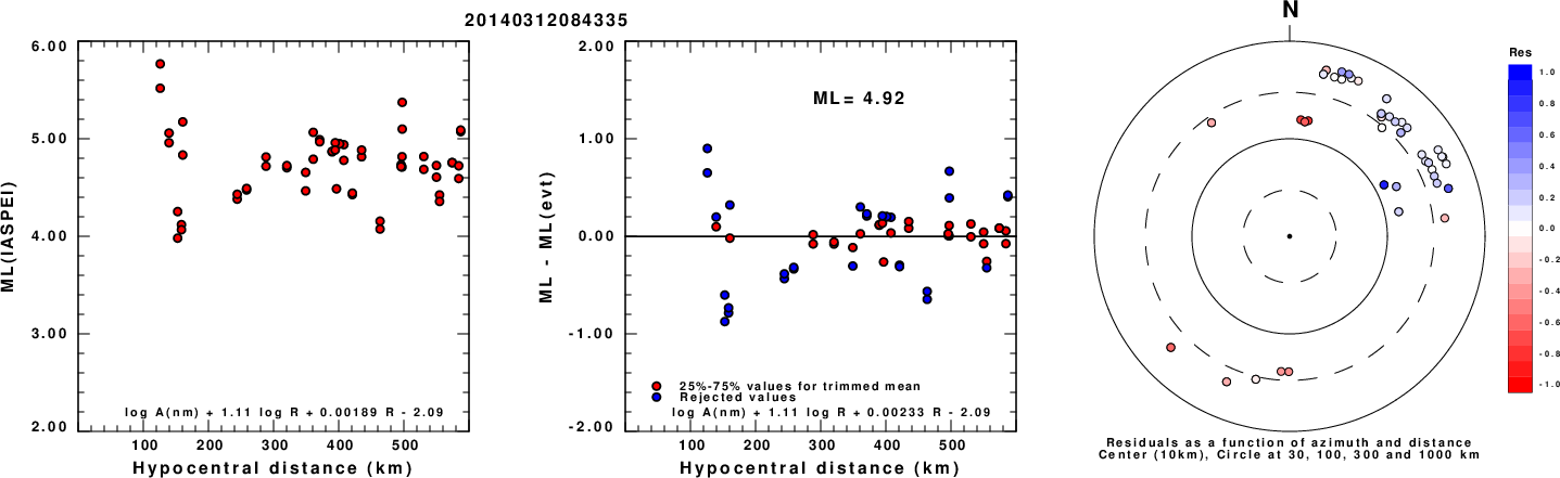
Left: ML computed using the IASPEI formula for Horizontal components. Center: ML residuals computed using a modified IASPEI formula that accounts for path specific attenuation; the values used for the trimmed mean are indicated. The ML relation used for each figure is given at the bottom of each plot.
Right: Residuals from new relation as a function of distance and azimuth.
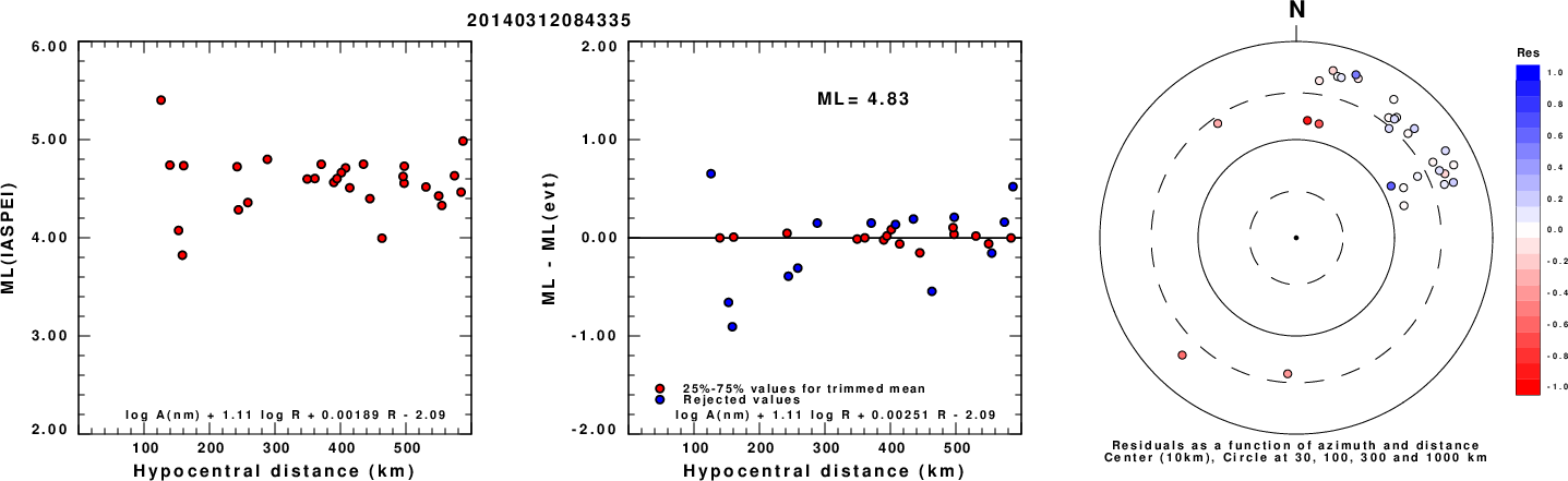
Left: ML computed using the IASPEI formula for Vertical components (research). Center: ML residuals computed using a modified IASPEI formula that accounts for path specific attenuation; the values used for the trimmed mean are indicated. The ML relation used for each figure is given at the bottom of each plot.
Right: Residuals from new relation as a function of distance and azimuth.
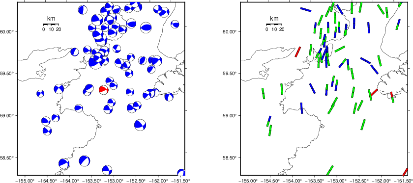
Context
The left panel of the next figure presents the focal mechanism for this earthquake (red) in the context of other nearby events (blue) in the SLU Moment Tensor Catalog. The right panel shows the inferred direction of maximum compressive stress and the type of faulting (green is strike-slip, red is normal, blue is thrust; oblique is shown by a combination of colors). Thus context plot is useful for assessing the appropriateness of the moment tensor of this event.
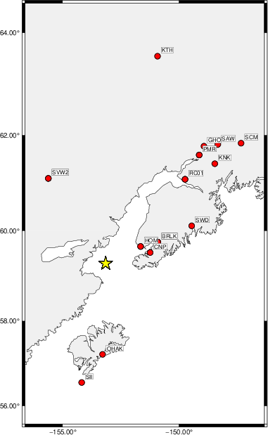
Waveform Inversion using wvfgrd96
The focal mechanism was determined using broadband seismic waveforms. The location of the event (star) and the
stations used for (red) the waveform inversion are shown in the next figure.
|
|
Location of broadband stations used for waveform inversion
|
The program wvfgrd96 was used with good traces observed at short distance to determine the focal mechanism, depth and seismic moment. This technique requires a high quality signal and well determined velocity model for the Green's functions. To the extent that these are the quality data, this type of mechanism should be preferred over the radiation pattern technique which requires the separate step of defining the pressure and tension quadrants and the correct strike.
The observed and predicted traces are filtered using the following gsac commands:
cut a -30 a 180
rtr
taper w 0.1
hp c 0.02 n 3
lp c 0.06 n 3
The results of this grid search are as follow:
           DEPTH  STK   DIP  RAKE   MW    FIT
WVFGRD96    0.5   340    80   -20   3.79 0.2283
WVFGRD96    1.0   165    85     5   3.81 0.2464
WVFGRD96    2.0   345    90   -10   3.92 0.3177
WVFGRD96    3.0   160    75   -15   3.96 0.3400
WVFGRD96    4.0   345    90   -15   3.99 0.3556
WVFGRD96    5.0   165    75    10   4.02 0.3670
WVFGRD96    6.0   165    75    10   4.04 0.3760
WVFGRD96    7.0   165    75    10   4.06 0.3804
WVFGRD96    8.0   255    85    -5   4.09 0.3966
WVFGRD96    9.0   255    85    -5   4.11 0.4125
WVFGRD96   10.0    80    90    10   4.15 0.4258
WVFGRD96   11.0    80    90     0   4.17 0.4388
WVFGRD96   12.0    80    90     0   4.18 0.4506
WVFGRD96   13.0    80    90     0   4.20 0.4612
WVFGRD96   14.0   255    90     0   4.20 0.4707
WVFGRD96   15.0    75    90     5   4.21 0.4794
WVFGRD96   16.0    75    90     0   4.22 0.4878
WVFGRD96   17.0    75    80     0   4.24 0.4975
WVFGRD96   18.0    75    80     0   4.25 0.5074
WVFGRD96   19.0    75    80     0   4.26 0.5171
WVFGRD96   20.0    75    80     0   4.27 0.5267
WVFGRD96   21.0    75    80     0   4.29 0.5357
WVFGRD96   22.0    75    80     0   4.30 0.5446
WVFGRD96   23.0    75    80     0   4.31 0.5540
WVFGRD96   24.0    75    80     0   4.32 0.5632
WVFGRD96   25.0    75    80     0   4.33 0.5726
WVFGRD96   26.0    75    80     0   4.34 0.5812
WVFGRD96   27.0    75    80     0   4.35 0.5889
WVFGRD96   28.0    75    80     0   4.36 0.5959
WVFGRD96   29.0    75    80     5   4.37 0.6027
WVFGRD96   30.0    75    80     5   4.38 0.6087
WVFGRD96   31.0    70    80     0   4.38 0.6145
WVFGRD96   32.0    70    80     0   4.39 0.6206
WVFGRD96   33.0    70    80     0   4.40 0.6258
WVFGRD96   34.0    70    80     0   4.41 0.6305
WVFGRD96   35.0    70    80     0   4.42 0.6351
WVFGRD96   36.0    70    80     0   4.43 0.6398
WVFGRD96   37.0    70    80     0   4.44 0.6440
WVFGRD96   38.0    70    80     0   4.46 0.6479
WVFGRD96   39.0    65    80     0   4.47 0.6513
WVFGRD96   40.0    65    75    -5   4.49 0.6554
WVFGRD96   41.0    65    75    -5   4.50 0.6561
WVFGRD96   42.0    65    75    -5   4.51 0.6565
WVFGRD96   43.0    65    75    -5   4.52 0.6569
WVFGRD96   44.0    65    75    -5   4.53 0.6576
WVFGRD96   45.0    65    75    -5   4.54 0.6582
WVFGRD96   46.0    65    75     5   4.54 0.6592
WVFGRD96   47.0    65    75     5   4.55 0.6608
WVFGRD96   48.0    65    75     5   4.55 0.6624
WVFGRD96   49.0    65    75     5   4.56 0.6639
WVFGRD96   50.0    65    75     5   4.57 0.6654
WVFGRD96   51.0    65    75    10   4.57 0.6669
WVFGRD96   52.0    65    80    15   4.58 0.6683
WVFGRD96   53.0    65    80    20   4.58 0.6700
WVFGRD96   54.0    65    80    20   4.59 0.6727
WVFGRD96   55.0    65    80    20   4.59 0.6749
WVFGRD96   56.0    65    80    20   4.60 0.6767
WVFGRD96   57.0    65    75    20   4.60 0.6783
WVFGRD96   58.0    65    80    25   4.61 0.6809
WVFGRD96   59.0    65    75    25   4.61 0.6841
WVFGRD96   60.0    65    75    25   4.62 0.6863
WVFGRD96   61.0    65    75    25   4.62 0.6872
WVFGRD96   62.0    65    75    30   4.63 0.6902
WVFGRD96   63.0    65    75    30   4.63 0.6932
WVFGRD96   64.0    65    75    30   4.63 0.6945
WVFGRD96   65.0    65    75    30   4.63 0.6963
WVFGRD96   66.0    65    75    35   4.64 0.6983
WVFGRD96   67.0    65    75    35   4.64 0.6995
WVFGRD96   68.0    65    75    35   4.65 0.7013
WVFGRD96   69.0    65    75    35   4.65 0.7028
WVFGRD96   70.0    65    75    35   4.65 0.7028
WVFGRD96   71.0    65    75    40   4.66 0.7056
WVFGRD96   72.0    65    75    40   4.66 0.7061
WVFGRD96   73.0    65    75    40   4.66 0.7061
WVFGRD96   74.0    65    75    40   4.66 0.7082
WVFGRD96   75.0    65    75    40   4.66 0.7073
WVFGRD96   76.0    65    75    40   4.66 0.7092
WVFGRD96   77.0    65    75    40   4.66 0.7092
WVFGRD96   78.0    65    75    40   4.66 0.7094
WVFGRD96   79.0    65    75    45   4.67 0.7102
WVFGRD96   80.0    65    75    45   4.67 0.7100
WVFGRD96   81.0    65    75    45   4.67 0.7100
WVFGRD96   82.0    65    75    45   4.68 0.7098
WVFGRD96   83.0    65    75    45   4.68 0.7106
WVFGRD96   84.0    65    75    45   4.68 0.7092
WVFGRD96   85.0    65    75    45   4.68 0.7106
WVFGRD96   86.0    65    75    45   4.68 0.7086
WVFGRD96   87.0    65    75    45   4.68 0.7101
WVFGRD96   88.0    65    75    45   4.68 0.7077
WVFGRD96   89.0    65    75    45   4.68 0.7096
WVFGRD96   90.0    65    75    45   4.68 0.7072
WVFGRD96   91.0    65    75    45   4.68 0.7086
WVFGRD96   92.0    65    75    50   4.69 0.7071
WVFGRD96   93.0    65    75    50   4.69 0.7072
WVFGRD96   94.0    65    75    50   4.69 0.7066
WVFGRD96   95.0    65    75    50   4.69 0.7062
WVFGRD96   96.0    65    75    50   4.69 0.7059
WVFGRD96   97.0    65    75    50   4.69 0.7048
WVFGRD96   98.0    65    75    50   4.69 0.7048
WVFGRD96   99.0    65    75    50   4.69 0.7030
The best solution is
WVFGRD96 85.0 65 75 45 4.68 0.7106
The mechanism corresponding to the best fit is
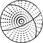
|
|
Figure 1. Waveform inversion focal mechanism
|
The best fit as a function of depth is given in the following figure:
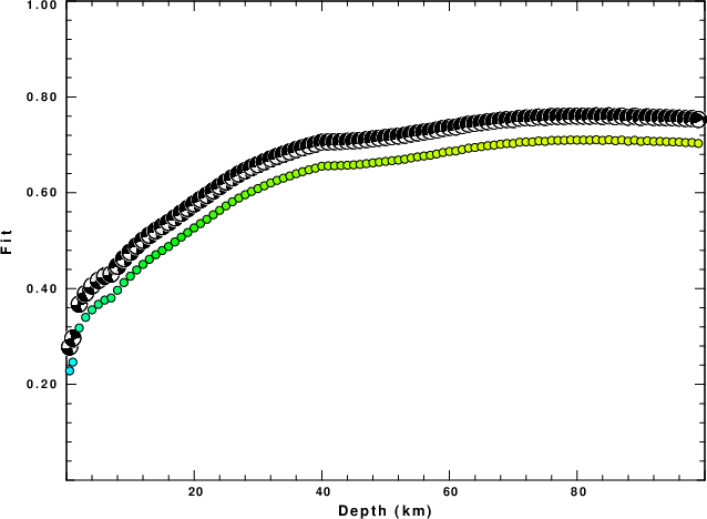
|
|
Figure 2. Depth sensitivity for waveform mechanism
|
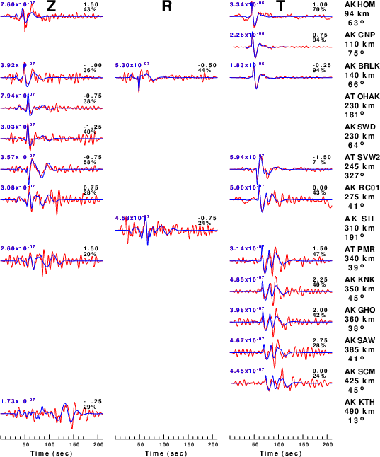
The comparison of the observed and predicted waveforms is given in the next figure. The red traces are the observed and the blue are the predicted.
Each observed-predicted component is plotted to the same scale and peak amplitudes are indicated by the numbers to the left of each trace. A pair of numbers is given in black at the right of each predicted traces. The upper number it the time shift required for maximum correlation between the observed and predicted traces. This time shift is required because the synthetics are not computed at exactly the same distance as the observed, the velocity model used in the predictions may not be perfect and the epicentral parameters may be be off.
A positive time shift indicates that the prediction is too fast and should be delayed to match the observed trace (shift to the right in this figure). A negative value indicates that the prediction is too slow. The lower number gives the percentage of variance reduction to characterize the individual goodness of fit (100% indicates a perfect fit).
The bandpass filter used in the processing and for the display was
cut a -30 a 180
rtr
taper w 0.1
hp c 0.02 n 3
lp c 0.06 n 3
|
|
Figure 3. Waveform comparison for selected depth. Red: observed; Blue - predicted. The time shift with respect to the model prediction is indicated. The percent of fit is also indicated. The time scale is relative to the first trace sample.
|
|
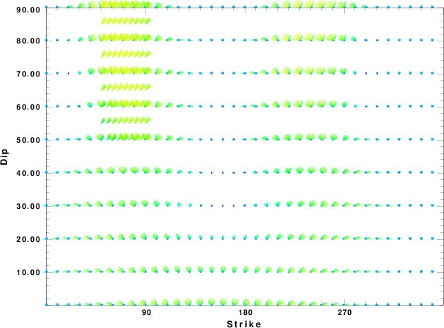
|
Focal mechanism sensitivity at the preferred depth. The red color indicates a very good fit to the waveforms.
Each solution is plotted as a vector at a given value of strike and dip with the angle of the vector representing the rake angle, measured, with respect to the upward vertical (N) in the figure.
|
A check on the assumed source location is possible by looking at the time shifts between the observed and predicted traces. The time shifts for waveform matching arise for several reasons:
- The origin time and epicentral distance are incorrect
- The velocity model used for the inversion is incorrect
- The velocity model used to define the P-arrival time is not the
same as the velocity model used for the waveform inversion
(assuming that the initial trace alignment is based on the
P arrival time)
Assuming only a mislocation, the time shifts are fit to a functional form:
Time_shift = A + B cos Azimuth + C Sin Azimuth
The time shifts for this inversion lead to the next figure:
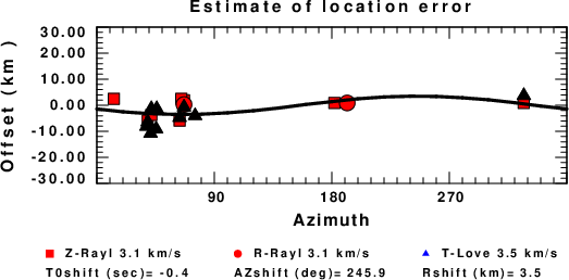
The derived shift in origin time and epicentral coordinates are given at the bottom of the figure.
Velocity Model
The WUS.model used for the waveform synthetic seismograms and for the surface wave eigenfunctions and dispersion is as follows
(The format is in the model96 format of Computer Programs in Seismology).
MODEL.01
Model after     8 iterations
ISOTROPIC
KGS
FLAT EARTH
1-D
CONSTANT VELOCITY
LINE08
LINE09
LINE10
LINE11
      H(KM)   VP(KM/S)   VS(KM/S) RHO(GM/CC)         QP         QS       ETAP       ETAS      FREFP      FREFS
     1.9000     3.4065     2.0089     2.2150  0.302E-02  0.679E-02   0.00       0.00       1.00       1.00
     6.1000     5.5445     3.2953     2.6089  0.349E-02  0.784E-02   0.00       0.00       1.00       1.00
    13.0000     6.2708     3.7396     2.7812  0.212E-02  0.476E-02   0.00       0.00       1.00       1.00
    19.0000     6.4075     3.7680     2.8223  0.111E-02  0.249E-02   0.00       0.00       1.00       1.00
     0.0000     7.9000     4.6200     3.2760  0.164E-10  0.370E-10   0.00       0.00       1.00       1.00
Last Changed Fri Apr 26 03:46:36 PM CDT 2024