Location
Location ANSS
The ANSS event ID is ak01434q4y01 and the event page is at
https://earthquake.usgs.gov/earthquakes/eventpage/ak01434q4y01/executive.
2014/03/09 16:11:23 61.030 -150.686 55.3 3.7 Alaska
Focal Mechanism
 USGS/SLU Moment Tensor Solution
 ENS  2014/03/09 16:11:23:0  61.03 -150.69  55.3 3.7 Alaska

 Stations used:
   AK.CRQ AK.DHY AK.GLB AK.GLI AK.KNK AK.MCK AK.RC01 AK.SAW
   AK.SCM AK.SKN AK.SSN AK.TGL AT.MENT AT.PMR AT.SVW2

 Filtering commands used:
   cut a -30 a 180
   rtr
   taper w 0.1
   hp c 0.02 n 3
   lp c 0.06 n 3

 Best Fitting Double Couple
  Mo = 1.02e+22 dyne-cm
  Mw = 3.94
  Z  = 58 km
  Plane   Strike  Dip  Rake
   NP1      190    75   -80
   NP2      336    18   -123
  Principal Axes:
   Axis    Value   Plunge  Azimuth
    T   1.02e+22     29     272
    N   0.00e+00     10       7
    P  -1.02e+22     59     114

 Moment Tensor: (dyne-cm)
    Component   Value
       Mxx    -4.35e+20
       Mxy     7.51e+20
       Mxz     1.97e+21
       Myy     5.47e+21
       Myz    -8.51e+21
       Mzz    -5.04e+21


                     -#####----####
                 #############----#####
              ###############--------#####
             ###############-----------####
           ################--------------####
          #################---------------####
         #################-----------------####
        #################-------------------####
        #################--------------------###
       #####   ##########--------------------####
       ##### T #########---------------------####
       #####   #########----------   ---------###
       #################---------- P ---------###
        ###############-----------   --------###
        ###############----------------------###
         ##############----------------------##
          #############---------------------##
           ############--------------------##
             ##########-------------------#
              #########-----------------##
                 #######--------------#
                     ###-----------


 Global CMT Convention Moment Tensor:
      R          T          P
 -5.04e+21   1.97e+21   8.51e+21
  1.97e+21  -4.35e+20  -7.51e+20
  8.51e+21  -7.51e+20   5.47e+21


Details of the solution is found at

http://www.eas.slu.edu/eqc/eqc_mt/MECH.NA/20140309161123/index.html
|
Preferred Solution
The preferred solution from an analysis of the surface-wave spectral amplitude radiation pattern, waveform inversion or first motion observations is
      STK = 190
      DIP = 75
     RAKE = -80
       MW = 3.94
       HS = 58.0
The NDK file is 20140309161123.ndk
The waveform inversion is preferred.
Moment Tensor Comparison
The following compares this source inversion to those provided by others. The purpose is to look for major differences and also to note slight differences that might be inherent to the processing procedure. For completeness the USGS/SLU solution is repeated from above.
| SLU |
USGSMT |
 USGS/SLU Moment Tensor Solution
 ENS  2014/03/09 16:11:23:0  61.03 -150.69  55.3 3.7 Alaska

 Stations used:
   AK.CRQ AK.DHY AK.GLB AK.GLI AK.KNK AK.MCK AK.RC01 AK.SAW
   AK.SCM AK.SKN AK.SSN AK.TGL AT.MENT AT.PMR AT.SVW2

 Filtering commands used:
   cut a -30 a 180
   rtr
   taper w 0.1
   hp c 0.02 n 3
   lp c 0.06 n 3

 Best Fitting Double Couple
  Mo = 1.02e+22 dyne-cm
  Mw = 3.94
  Z  = 58 km
  Plane   Strike  Dip  Rake
   NP1      190    75   -80
   NP2      336    18   -123
  Principal Axes:
   Axis    Value   Plunge  Azimuth
    T   1.02e+22     29     272
    N   0.00e+00     10       7
    P  -1.02e+22     59     114

 Moment Tensor: (dyne-cm)
    Component   Value
       Mxx    -4.35e+20
       Mxy     7.51e+20
       Mxz     1.97e+21
       Myy     5.47e+21
       Myz    -8.51e+21
       Mzz    -5.04e+21


                     -#####----####
                 #############----#####
              ###############--------#####
             ###############-----------####
           ################--------------####
          #################---------------####
         #################-----------------####
        #################-------------------####
        #################--------------------###
       #####   ##########--------------------####
       ##### T #########---------------------####
       #####   #########----------   ---------###
       #################---------- P ---------###
        ###############-----------   --------###
        ###############----------------------###
         ##############----------------------##
          #############---------------------##
           ############--------------------##
             ##########-------------------#
              #########-----------------##
                 #######--------------#
                     ###-----------


 Global CMT Convention Moment Tensor:
      R          T          P
 -5.04e+21   1.97e+21   8.51e+21
  1.97e+21  -4.35e+20  -7.51e+20
  8.51e+21  -7.51e+20   5.47e+21


Details of the solution is found at

http://www.eas.slu.edu/eqc/eqc_mt/MECH.NA/20140309161123/index.html
|
Moment
    1.06e+15 N-m
Magnitude
    4.0
Percent DC
    71%
Depth
    58.0 km
Updated
    2014-03-09 17:31:46 UTC
Author
    us
Catalog
    ak
Contributor
    us
Code
    us_c000n5yj_mwr

Principal Axes
Axis	Value	Plunge	Azimuth
T	0.987	33°	277°
N	0.139	7°	12°
P	-1.126	56°	113°
Nodal Planes
Plane	Strike	Dip	Rake
NP1	194°	78°	-82°
NP2	341°	14°	-122°
|
|
Magnitudes
Given the availability of digital waveforms for determination of the moment tensor, this section documents the added processing leading to mLg, if appropriate to the region, and ML by application of the respective IASPEI formulae. As a research study, the linear distance term of the IASPEI formula
for ML is adjusted to remove a linear distance trend in residuals to give a regionally defined ML. The defined ML uses horizontal component recordings, but the same procedure is applied to the vertical components since there may be some interest in vertical component ground motions. Residual plots versus distance may indicate interesting features of ground motion scaling in some distance ranges. A residual plot of the regionalized magnitude is given as a function of distance and azimuth, since data sets may transcend different wave propagation provinces.
ML Magnitude
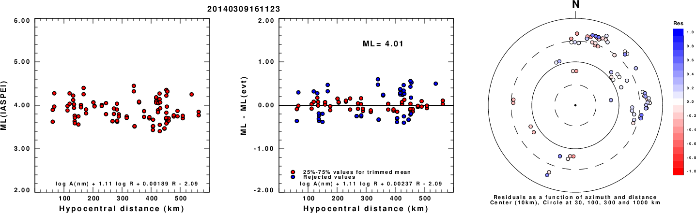
Left: ML computed using the IASPEI formula for Horizontal components. Center: ML residuals computed using a modified IASPEI formula that accounts for path specific attenuation; the values used for the trimmed mean are indicated. The ML relation used for each figure is given at the bottom of each plot.
Right: Residuals from new relation as a function of distance and azimuth.
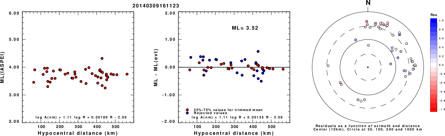
Left: ML computed using the IASPEI formula for Vertical components (research). Center: ML residuals computed using a modified IASPEI formula that accounts for path specific attenuation; the values used for the trimmed mean are indicated. The ML relation used for each figure is given at the bottom of each plot.
Right: Residuals from new relation as a function of distance and azimuth.
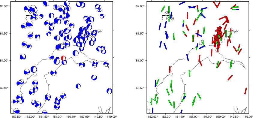
Context
The left panel of the next figure presents the focal mechanism for this earthquake (red) in the context of other nearby events (blue) in the SLU Moment Tensor Catalog. The right panel shows the inferred direction of maximum compressive stress and the type of faulting (green is strike-slip, red is normal, blue is thrust; oblique is shown by a combination of colors). Thus context plot is useful for assessing the appropriateness of the moment tensor of this event.
Waveform Inversion using wvfgrd96
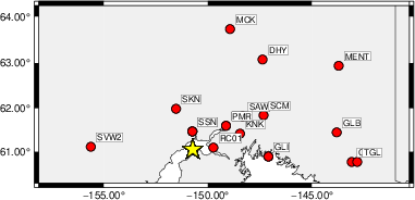
The focal mechanism was determined using broadband seismic waveforms. The location of the event (star) and the
stations used for (red) the waveform inversion are shown in the next figure.
|
|
Location of broadband stations used for waveform inversion
|
The program wvfgrd96 was used with good traces observed at short distance to determine the focal mechanism, depth and seismic moment. This technique requires a high quality signal and well determined velocity model for the Green's functions. To the extent that these are the quality data, this type of mechanism should be preferred over the radiation pattern technique which requires the separate step of defining the pressure and tension quadrants and the correct strike.
The observed and predicted traces are filtered using the following gsac commands:
cut a -30 a 180
rtr
taper w 0.1
hp c 0.02 n 3
lp c 0.06 n 3
The results of this grid search are as follow:
           DEPTH  STK   DIP  RAKE   MW    FIT
WVFGRD96    0.5   200    80   -10   3.10 0.1446
WVFGRD96    1.0   200    80   -10   3.14 0.1586
WVFGRD96    2.0   200    80   -15   3.25 0.2018
WVFGRD96    3.0   195    65   -20   3.34 0.2339
WVFGRD96    4.0   200    75   -15   3.37 0.2537
WVFGRD96    5.0   200    75    -5   3.41 0.2663
WVFGRD96    6.0   200    80     0   3.44 0.2745
WVFGRD96    7.0   200    80     0   3.46 0.2808
WVFGRD96    8.0   200    75    10   3.50 0.2899
WVFGRD96    9.0   200    75    10   3.51 0.2952
WVFGRD96   10.0   200    75    10   3.53 0.2960
WVFGRD96   11.0   200    80    10   3.54 0.2943
WVFGRD96   12.0   200    80    10   3.55 0.2925
WVFGRD96   13.0   200    80    20   3.56 0.2931
WVFGRD96   14.0   200    80    20   3.57 0.2970
WVFGRD96   15.0    20    85    35   3.55 0.3023
WVFGRD96   16.0    20    85    35   3.55 0.3098
WVFGRD96   17.0    20    90    35   3.56 0.3171
WVFGRD96   18.0    20    90    35   3.57 0.3244
WVFGRD96   19.0    20    90    35   3.57 0.3316
WVFGRD96   20.0   195    85   -35   3.59 0.3404
WVFGRD96   21.0    20    90    40   3.59 0.3447
WVFGRD96   22.0    20    90    40   3.60 0.3518
WVFGRD96   23.0    20    90    40   3.60 0.3589
WVFGRD96   24.0    20    90    40   3.61 0.3656
WVFGRD96   25.0   195    85   -40   3.62 0.3730
WVFGRD96   26.0    20    90    45   3.62 0.3785
WVFGRD96   27.0    20    90    45   3.63 0.3853
WVFGRD96   28.0    20    90    45   3.64 0.3917
WVFGRD96   29.0    20    90    50   3.65 0.3985
WVFGRD96   30.0   195    85   -50   3.65 0.4079
WVFGRD96   31.0    20    90    50   3.66 0.4116
WVFGRD96   32.0   195    85   -50   3.67 0.4210
WVFGRD96   33.0   195    85   -55   3.68 0.4271
WVFGRD96   34.0   195    85   -55   3.68 0.4328
WVFGRD96   35.0   195    85   -55   3.69 0.4380
WVFGRD96   36.0   195    80   -55   3.69 0.4426
WVFGRD96   37.0   195    80   -55   3.70 0.4480
WVFGRD96   38.0   195    80   -60   3.70 0.4519
WVFGRD96   39.0   195    80   -55   3.71 0.4558
WVFGRD96   40.0   195    80   -65   3.84 0.4557
WVFGRD96   41.0   195    80   -65   3.84 0.4600
WVFGRD96   42.0   195    80   -65   3.85 0.4635
WVFGRD96   43.0   195    80   -70   3.86 0.4672
WVFGRD96   44.0   195    80   -70   3.86 0.4702
WVFGRD96   45.0   195    80   -70   3.87 0.4728
WVFGRD96   46.0   195    80   -70   3.87 0.4760
WVFGRD96   47.0   195    80   -70   3.88 0.4778
WVFGRD96   48.0   190    75   -70   3.88 0.4805
WVFGRD96   49.0   190    75   -70   3.89 0.4828
WVFGRD96   50.0   190    75   -70   3.89 0.4849
WVFGRD96   51.0   190    75   -75   3.90 0.4872
WVFGRD96   52.0   190    75   -75   3.91 0.4888
WVFGRD96   53.0   190    75   -75   3.91 0.4907
WVFGRD96   54.0   190    75   -75   3.92 0.4916
WVFGRD96   55.0   190    75   -75   3.92 0.4925
WVFGRD96   56.0   190    75   -80   3.93 0.4930
WVFGRD96   57.0   190    75   -80   3.93 0.4935
WVFGRD96   58.0   190    75   -80   3.94 0.4937
WVFGRD96   59.0   190    75   -80   3.94 0.4929
WVFGRD96   60.0     0    15  -100   3.95 0.4920
WVFGRD96   61.0   190    75   -85   3.95 0.4914
WVFGRD96   62.0     0    15  -100   3.96 0.4907
WVFGRD96   63.0    10    15   -90   3.97 0.4888
WVFGRD96   64.0    10    15   -90   3.97 0.4874
WVFGRD96   65.0    10    15   -90   3.97 0.4860
WVFGRD96   66.0    45    15   -60   3.99 0.4841
WVFGRD96   67.0    45    15   -60   3.99 0.4829
WVFGRD96   68.0    45    15   -60   3.99 0.4817
WVFGRD96   69.0    60    15   -50   4.00 0.4794
WVFGRD96   70.0    50    15   -55   4.00 0.4784
WVFGRD96   71.0    65    15   -45   4.01 0.4767
WVFGRD96   72.0    65    15   -45   4.01 0.4743
WVFGRD96   73.0    65    15   -45   4.01 0.4727
WVFGRD96   74.0    75    20   -35   4.03 0.4700
WVFGRD96   75.0    75    20   -35   4.03 0.4680
WVFGRD96   76.0    75    20   -35   4.03 0.4662
WVFGRD96   77.0    75    20   -35   4.03 0.4634
WVFGRD96   78.0    85    20   -30   4.04 0.4611
WVFGRD96   79.0    85    20   -30   4.04 0.4591
WVFGRD96   80.0    90    25   -25   4.06 0.4564
WVFGRD96   81.0    90    25   -25   4.06 0.4545
WVFGRD96   82.0    90    25   -25   4.06 0.4527
WVFGRD96   83.0    90    25   -25   4.07 0.4502
WVFGRD96   84.0    90    25   -25   4.07 0.4472
WVFGRD96   85.0    90    25   -25   4.07 0.4450
WVFGRD96   86.0    90    25   -25   4.07 0.4422
WVFGRD96   87.0    95    30   -20   4.09 0.4387
WVFGRD96   88.0    95    30   -20   4.09 0.4370
WVFGRD96   89.0    95    30   -20   4.09 0.4345
WVFGRD96   90.0    95    30   -20   4.09 0.4320
WVFGRD96   91.0    95    30   -20   4.09 0.4291
WVFGRD96   92.0    95    30   -20   4.10 0.4268
WVFGRD96   93.0    95    30   -20   4.10 0.4238
WVFGRD96   94.0    95    30   -20   4.10 0.4206
WVFGRD96   95.0   100    30   -20   4.11 0.4177
WVFGRD96   96.0   100    35   -20   4.12 0.4151
WVFGRD96   97.0   100    35   -20   4.12 0.4126
WVFGRD96   98.0   105    35   -15   4.13 0.4099
WVFGRD96   99.0   105    35   -15   4.13 0.4079
The best solution is
WVFGRD96 58.0 190 75 -80 3.94 0.4937
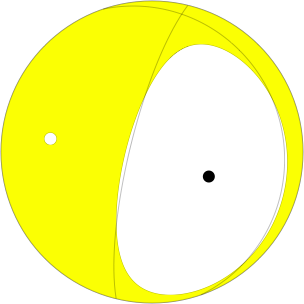
The mechanism corresponding to the best fit is
|
|
Figure 1. Waveform inversion focal mechanism
|
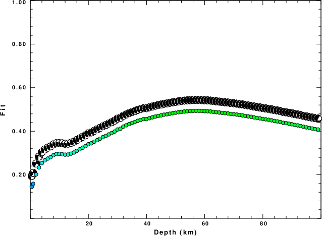
The best fit as a function of depth is given in the following figure:
|
|
Figure 2. Depth sensitivity for waveform mechanism
|
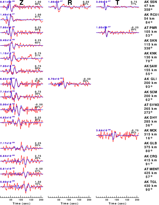
The comparison of the observed and predicted waveforms is given in the next figure. The red traces are the observed and the blue are the predicted.
Each observed-predicted component is plotted to the same scale and peak amplitudes are indicated by the numbers to the left of each trace. A pair of numbers is given in black at the right of each predicted traces. The upper number it the time shift required for maximum correlation between the observed and predicted traces. This time shift is required because the synthetics are not computed at exactly the same distance as the observed, the velocity model used in the predictions may not be perfect and the epicentral parameters may be be off.
A positive time shift indicates that the prediction is too fast and should be delayed to match the observed trace (shift to the right in this figure). A negative value indicates that the prediction is too slow. The lower number gives the percentage of variance reduction to characterize the individual goodness of fit (100% indicates a perfect fit).
The bandpass filter used in the processing and for the display was
cut a -30 a 180
rtr
taper w 0.1
hp c 0.02 n 3
lp c 0.06 n 3
|
|
Figure 3. Waveform comparison for selected depth. Red: observed; Blue - predicted. The time shift with respect to the model prediction is indicated. The percent of fit is also indicated. The time scale is relative to the first trace sample.
|
|
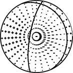
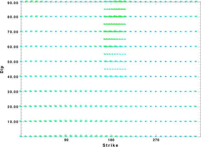
|
Focal mechanism sensitivity at the preferred depth. The red color indicates a very good fit to the waveforms.
Each solution is plotted as a vector at a given value of strike and dip with the angle of the vector representing the rake angle, measured, with respect to the upward vertical (N) in the figure.
|
A check on the assumed source location is possible by looking at the time shifts between the observed and predicted traces. The time shifts for waveform matching arise for several reasons:
- The origin time and epicentral distance are incorrect
- The velocity model used for the inversion is incorrect
- The velocity model used to define the P-arrival time is not the
same as the velocity model used for the waveform inversion
(assuming that the initial trace alignment is based on the
P arrival time)
Assuming only a mislocation, the time shifts are fit to a functional form:
Time_shift = A + B cos Azimuth + C Sin Azimuth
The time shifts for this inversion lead to the next figure:
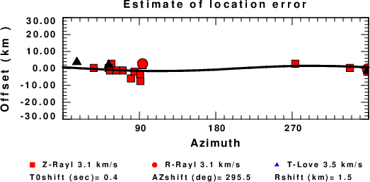
The derived shift in origin time and epicentral coordinates are given at the bottom of the figure.
Velocity Model
The WUS.model used for the waveform synthetic seismograms and for the surface wave eigenfunctions and dispersion is as follows
(The format is in the model96 format of Computer Programs in Seismology).
MODEL.01
Model after     8 iterations
ISOTROPIC
KGS
FLAT EARTH
1-D
CONSTANT VELOCITY
LINE08
LINE09
LINE10
LINE11
      H(KM)   VP(KM/S)   VS(KM/S) RHO(GM/CC)         QP         QS       ETAP       ETAS      FREFP      FREFS
     1.9000     3.4065     2.0089     2.2150  0.302E-02  0.679E-02   0.00       0.00       1.00       1.00
     6.1000     5.5445     3.2953     2.6089  0.349E-02  0.784E-02   0.00       0.00       1.00       1.00
    13.0000     6.2708     3.7396     2.7812  0.212E-02  0.476E-02   0.00       0.00       1.00       1.00
    19.0000     6.4075     3.7680     2.8223  0.111E-02  0.249E-02   0.00       0.00       1.00       1.00
     0.0000     7.9000     4.6200     3.2760  0.164E-10  0.370E-10   0.00       0.00       1.00       1.00
Last Changed Fri Apr 26 03:37:39 PM CDT 2024