Location
Location ANSS
The ANSS event ID is ak0142xw9c94 and the event page is at
https://earthquake.usgs.gov/earthquakes/eventpage/ak0142xw9c94/executive.
2014/03/05 03:13:19 62.081 -149.458 38.4 4.4 Alaska
Focal Mechanism
 USGS/SLU Moment Tensor Solution
 ENS  2014/03/05 03:13:19:0  62.08 -149.46  38.4 4.4 Alaska

 Stations used:
   AK.BPAW AK.CCB AK.CRQ AK.DHY AK.FID AK.GHO AK.GLI AK.KNK
   AK.KTH AK.RIDG AK.RND AK.SAW AK.SCM AK.SCRK AK.SSN AK.TGL
   AK.TRF AK.WRH IU.COLA US.EGAK

 Filtering commands used:
   cut a -30 a 140
   rtr
   taper w 0.1
   hp c 0.02 n 3
   lp c 0.06 n 3

 Best Fitting Double Couple
  Mo = 4.07e+22 dyne-cm
  Mw = 4.34
  Z  = 52 km
  Plane   Strike  Dip  Rake
   NP1      200    65   -75
   NP2      348    29   -119
  Principal Axes:
   Axis    Value   Plunge  Azimuth
    T   4.07e+22     19     279
    N   0.00e+00     14      14
    P  -4.07e+22     67     137

 Moment Tensor: (dyne-cm)
    Component   Value
       Mxx    -2.62e+21
       Mxy    -2.37e+21
       Mxz     1.28e+22
       Myy     3.28e+22
       Myz    -2.22e+22
       Mzz    -3.01e+22


                     #######-------
                 ######################
              ################-----#######
             ###############---------######
           ################------------######
          ################--------------######
         ################----------------######
        ################------------------######
        ##   ##########-------------------######
       ### T #########---------------------######
       ###   #########---------------------######
       ##############----------------------######
       ##############----------   ---------######
        ############----------- P ---------#####
        ############-----------   ---------#####
         ###########----------------------#####
          #########----------------------#####
           ########----------------------####
             #######--------------------###
              ######------------------####
                 ###----------------###
                     -------------#


 Global CMT Convention Moment Tensor:
      R          T          P
 -3.01e+22   1.28e+22   2.22e+22
  1.28e+22  -2.62e+21   2.37e+21
  2.22e+22   2.37e+21   3.28e+22


Details of the solution is found at

http://www.eas.slu.edu/eqc/eqc_mt/MECH.NA/20140305031319/index.html
|
Preferred Solution
The preferred solution from an analysis of the surface-wave spectral amplitude radiation pattern, waveform inversion or first motion observations is
      STK = 200
      DIP = 65
     RAKE = -75
       MW = 4.34
       HS = 52.0
The NDK file is 20140305031319.ndk
The waveform inversion is preferred.
Moment Tensor Comparison
The following compares this source inversion to those provided by others. The purpose is to look for major differences and also to note slight differences that might be inherent to the processing procedure. For completeness the USGS/SLU solution is repeated from above.
| SLU |
USGSMT |
 USGS/SLU Moment Tensor Solution
 ENS  2014/03/05 03:13:19:0  62.08 -149.46  38.4 4.4 Alaska

 Stations used:
   AK.BPAW AK.CCB AK.CRQ AK.DHY AK.FID AK.GHO AK.GLI AK.KNK
   AK.KTH AK.RIDG AK.RND AK.SAW AK.SCM AK.SCRK AK.SSN AK.TGL
   AK.TRF AK.WRH IU.COLA US.EGAK

 Filtering commands used:
   cut a -30 a 140
   rtr
   taper w 0.1
   hp c 0.02 n 3
   lp c 0.06 n 3

 Best Fitting Double Couple
  Mo = 4.07e+22 dyne-cm
  Mw = 4.34
  Z  = 52 km
  Plane   Strike  Dip  Rake
   NP1      200    65   -75
   NP2      348    29   -119
  Principal Axes:
   Axis    Value   Plunge  Azimuth
    T   4.07e+22     19     279
    N   0.00e+00     14      14
    P  -4.07e+22     67     137

 Moment Tensor: (dyne-cm)
    Component   Value
       Mxx    -2.62e+21
       Mxy    -2.37e+21
       Mxz     1.28e+22
       Myy     3.28e+22
       Myz    -2.22e+22
       Mzz    -3.01e+22


                     #######-------
                 ######################
              ################-----#######
             ###############---------######
           ################------------######
          ################--------------######
         ################----------------######
        ################------------------######
        ##   ##########-------------------######
       ### T #########---------------------######
       ###   #########---------------------######
       ##############----------------------######
       ##############----------   ---------######
        ############----------- P ---------#####
        ############-----------   ---------#####
         ###########----------------------#####
          #########----------------------#####
           ########----------------------####
             #######--------------------###
              ######------------------####
                 ###----------------###
                     -------------#


 Global CMT Convention Moment Tensor:
      R          T          P
 -3.01e+22   1.28e+22   2.22e+22
  1.28e+22  -2.62e+21   2.37e+21
  2.22e+22   2.37e+21   3.28e+22


Details of the solution is found at

http://www.eas.slu.edu/eqc/eqc_mt/MECH.NA/20140305031319/index.html
|
Moment      4.08e+15 N-m
Magnitude   4.3
Percent DC  97%
Depth       51.0 km
Updated     2014-03-05 03:27:44 UTC
Author      us
Catalog     ak
Contributor us
Code        us_b000n1bg_mwr

Principal Axes
Axis	Value	Plunge	Azimuth
T	4.058	17	276
N	0.046	15	10
P	-4.104	67	140
Nodal Planes
Plane	Strike	Dip	Rake
NP1	198	64	-73
NP2	344	31	-120
|
|
Magnitudes
Given the availability of digital waveforms for determination of the moment tensor, this section documents the added processing leading to mLg, if appropriate to the region, and ML by application of the respective IASPEI formulae. As a research study, the linear distance term of the IASPEI formula
for ML is adjusted to remove a linear distance trend in residuals to give a regionally defined ML. The defined ML uses horizontal component recordings, but the same procedure is applied to the vertical components since there may be some interest in vertical component ground motions. Residual plots versus distance may indicate interesting features of ground motion scaling in some distance ranges. A residual plot of the regionalized magnitude is given as a function of distance and azimuth, since data sets may transcend different wave propagation provinces.
ML Magnitude
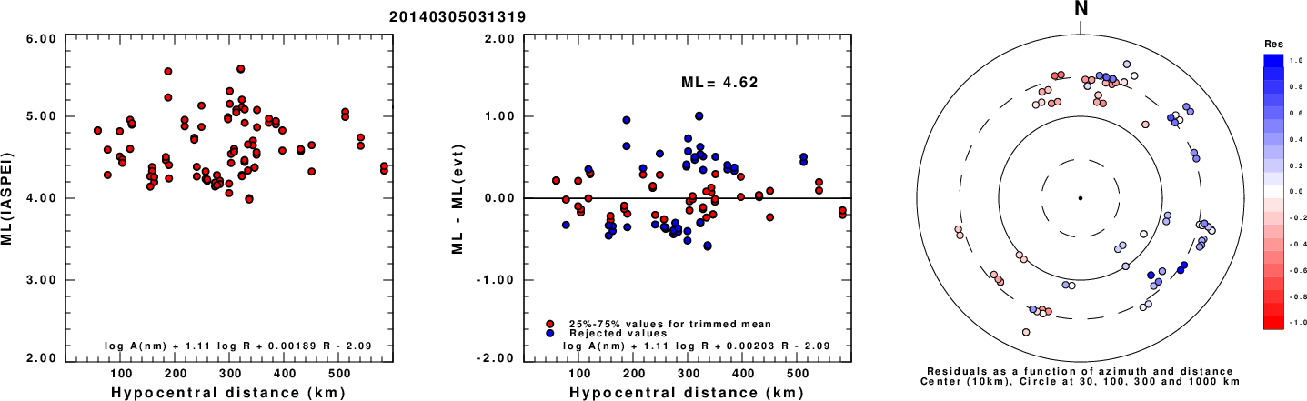
Left: ML computed using the IASPEI formula for Horizontal components. Center: ML residuals computed using a modified IASPEI formula that accounts for path specific attenuation; the values used for the trimmed mean are indicated. The ML relation used for each figure is given at the bottom of each plot.
Right: Residuals from new relation as a function of distance and azimuth.
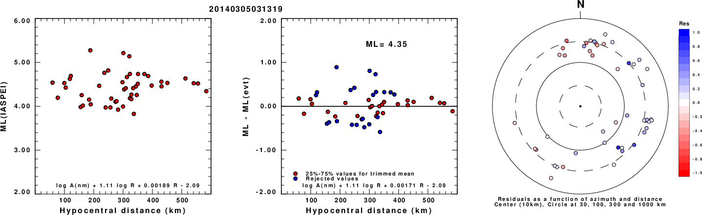
Left: ML computed using the IASPEI formula for Vertical components (research). Center: ML residuals computed using a modified IASPEI formula that accounts for path specific attenuation; the values used for the trimmed mean are indicated. The ML relation used for each figure is given at the bottom of each plot.
Right: Residuals from new relation as a function of distance and azimuth.
Context
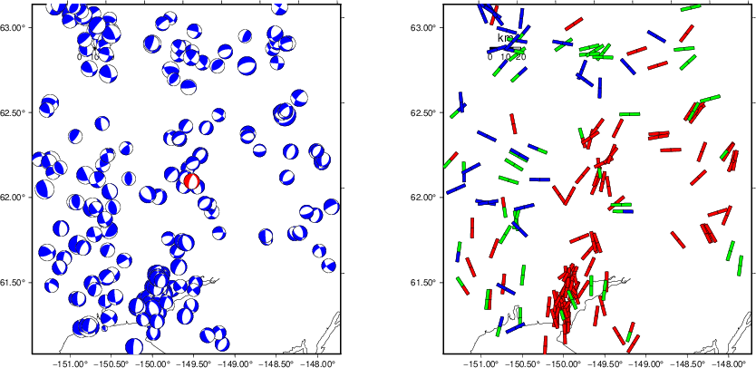
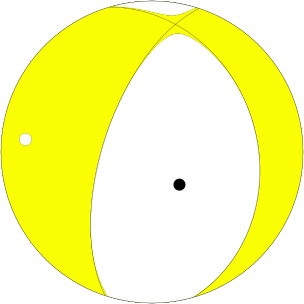
The left panel of the next figure presents the focal mechanism for this earthquake (red) in the context of other nearby events (blue) in the SLU Moment Tensor Catalog. The right panel shows the inferred direction of maximum compressive stress and the type of faulting (green is strike-slip, red is normal, blue is thrust; oblique is shown by a combination of colors). Thus context plot is useful for assessing the appropriateness of the moment tensor of this event.
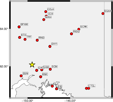
Waveform Inversion using wvfgrd96
The focal mechanism was determined using broadband seismic waveforms. The location of the event (star) and the
stations used for (red) the waveform inversion are shown in the next figure.
|
|
Location of broadband stations used for waveform inversion
|
The program wvfgrd96 was used with good traces observed at short distance to determine the focal mechanism, depth and seismic moment. This technique requires a high quality signal and well determined velocity model for the Green's functions. To the extent that these are the quality data, this type of mechanism should be preferred over the radiation pattern technique which requires the separate step of defining the pressure and tension quadrants and the correct strike.
The observed and predicted traces are filtered using the following gsac commands:
cut a -30 a 140
rtr
taper w 0.1
hp c 0.02 n 3
lp c 0.06 n 3
The results of this grid search are as follow:
           DEPTH  STK   DIP  RAKE   MW    FIT
WVFGRD96    2.0    20    40   -85   3.68 0.2842
WVFGRD96    4.0    75    65    -5   3.71 0.2775
WVFGRD96    6.0    75    65    15   3.76 0.3019
WVFGRD96    8.0    65    85    45   3.80 0.3381
WVFGRD96   10.0    65    80    45   3.82 0.3794
WVFGRD96   12.0    60    75    45   3.84 0.4146
WVFGRD96   14.0    55    75    45   3.87 0.4456
WVFGRD96   16.0    55    75    45   3.88 0.4698
WVFGRD96   18.0    55    75    40   3.91 0.4899
WVFGRD96   20.0   220    75   -45   3.92 0.5140
WVFGRD96   22.0   215    70   -45   3.96 0.5346
WVFGRD96   24.0   215    70   -45   3.98 0.5548
WVFGRD96   26.0   215    70   -45   4.00 0.5742
WVFGRD96   28.0   215    70   -45   4.02 0.5917
WVFGRD96   30.0   210    65   -50   4.04 0.6114
WVFGRD96   32.0   210    65   -55   4.06 0.6313
WVFGRD96   34.0   210    65   -55   4.08 0.6468
WVFGRD96   36.0   205    60   -60   4.11 0.6575
WVFGRD96   38.0   205    60   -60   4.13 0.6641
WVFGRD96   40.0   205    60   -70   4.24 0.6820
WVFGRD96   42.0   195    65   -80   4.26 0.6950
WVFGRD96   44.0   195    60   -80   4.28 0.7064
WVFGRD96   46.0   195    65   -80   4.29 0.7153
WVFGRD96   48.0   195    65   -80   4.31 0.7218
WVFGRD96   50.0   200    65   -75   4.32 0.7258
WVFGRD96   52.0   200    65   -75   4.34 0.7267
WVFGRD96   54.0   200    65   -70   4.35 0.7244
WVFGRD96   56.0   200    65   -70   4.36 0.7191
WVFGRD96   58.0   200    65   -70   4.37 0.7106
WVFGRD96   60.0   200    65   -70   4.38 0.6988
WVFGRD96   62.0   200    70   -70   4.38 0.6868
WVFGRD96   64.0   200    70   -70   4.39 0.6748
WVFGRD96   66.0   200    70   -70   4.39 0.6625
WVFGRD96   68.0   200    70   -70   4.40 0.6493
WVFGRD96   70.0   205    75   -65   4.40 0.6345
WVFGRD96   72.0   195    75   -80   4.40 0.6244
WVFGRD96   74.0   200    80   -75   4.40 0.6163
WVFGRD96   76.0   200    80   -75   4.41 0.6125
WVFGRD96   78.0   200    80   -75   4.41 0.6070
WVFGRD96   80.0   200    80   -75   4.42 0.6001
WVFGRD96   82.0   200    80   -75   4.42 0.5911
WVFGRD96   84.0   200    85   -75   4.42 0.5863
WVFGRD96   86.0   200    85   -75   4.43 0.5810
WVFGRD96   88.0    20    90    75   4.42 0.5615
WVFGRD96   90.0    20    90    75   4.43 0.5584
WVFGRD96   92.0    20    90    75   4.43 0.5541
WVFGRD96   94.0    20    90    75   4.43 0.5488
WVFGRD96   96.0   200    90   -70   4.44 0.5429
WVFGRD96   98.0    20    90    70   4.44 0.5369
WVFGRD96  100.0   200    90   -70   4.44 0.5294
The best solution is
WVFGRD96 52.0 200 65 -75 4.34 0.7267
The mechanism corresponding to the best fit is
|
|
Figure 1. Waveform inversion focal mechanism
|
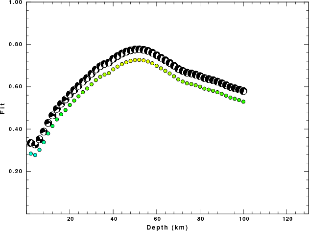
The best fit as a function of depth is given in the following figure:
|
|
Figure 2. Depth sensitivity for waveform mechanism
|
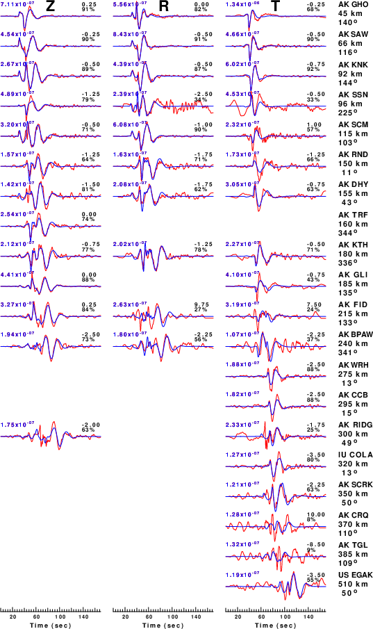
The comparison of the observed and predicted waveforms is given in the next figure. The red traces are the observed and the blue are the predicted.
Each observed-predicted component is plotted to the same scale and peak amplitudes are indicated by the numbers to the left of each trace. A pair of numbers is given in black at the right of each predicted traces. The upper number it the time shift required for maximum correlation between the observed and predicted traces. This time shift is required because the synthetics are not computed at exactly the same distance as the observed, the velocity model used in the predictions may not be perfect and the epicentral parameters may be be off.
A positive time shift indicates that the prediction is too fast and should be delayed to match the observed trace (shift to the right in this figure). A negative value indicates that the prediction is too slow. The lower number gives the percentage of variance reduction to characterize the individual goodness of fit (100% indicates a perfect fit).
The bandpass filter used in the processing and for the display was
cut a -30 a 140
rtr
taper w 0.1
hp c 0.02 n 3
lp c 0.06 n 3
|
|
Figure 3. Waveform comparison for selected depth. Red: observed; Blue - predicted. The time shift with respect to the model prediction is indicated. The percent of fit is also indicated. The time scale is relative to the first trace sample.
|
|
|
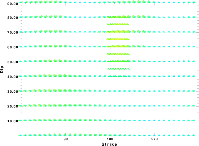
Focal mechanism sensitivity at the preferred depth. The red color indicates a very good fit to the waveforms.
Each solution is plotted as a vector at a given value of strike and dip with the angle of the vector representing the rake angle, measured, with respect to the upward vertical (N) in the figure.
|
A check on the assumed source location is possible by looking at the time shifts between the observed and predicted traces. The time shifts for waveform matching arise for several reasons:
- The origin time and epicentral distance are incorrect
- The velocity model used for the inversion is incorrect
- The velocity model used to define the P-arrival time is not the
same as the velocity model used for the waveform inversion
(assuming that the initial trace alignment is based on the
P arrival time)
Assuming only a mislocation, the time shifts are fit to a functional form:
Time_shift = A + B cos Azimuth + C Sin Azimuth
The time shifts for this inversion lead to the next figure:
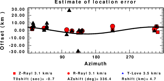
The derived shift in origin time and epicentral coordinates are given at the bottom of the figure.
Velocity Model
The WUS.model used for the waveform synthetic seismograms and for the surface wave eigenfunctions and dispersion is as follows
(The format is in the model96 format of Computer Programs in Seismology).
MODEL.01
Model after     8 iterations
ISOTROPIC
KGS
FLAT EARTH
1-D
CONSTANT VELOCITY
LINE08
LINE09
LINE10
LINE11
      H(KM)   VP(KM/S)   VS(KM/S) RHO(GM/CC)         QP         QS       ETAP       ETAS      FREFP      FREFS
     1.9000     3.4065     2.0089     2.2150  0.302E-02  0.679E-02   0.00       0.00       1.00       1.00
     6.1000     5.5445     3.2953     2.6089  0.349E-02  0.784E-02   0.00       0.00       1.00       1.00
    13.0000     6.2708     3.7396     2.7812  0.212E-02  0.476E-02   0.00       0.00       1.00       1.00
    19.0000     6.4075     3.7680     2.8223  0.111E-02  0.249E-02   0.00       0.00       1.00       1.00
     0.0000     7.9000     4.6200     3.2760  0.164E-10  0.370E-10   0.00       0.00       1.00       1.00
Last Changed Fri Apr 26 03:27:32 PM CDT 2024