Location

Location ANSS

The ANSS event ID is ak0141fma9kq and the event page is at https://earthquake.usgs.gov/earthquakes/eventpage/ak0141fma9kq/executive.

2014/01/31 21:20:54 58.118 -151.755 49.2 4.2 Alaska

Focal Mechanism

USGS/SLU Moment Tensor Solution ENS 2014/01/31 21:20:54:0 58.12 -151.76 49.2 4.2 Alaska Stations used: AK.BRLK AK.BRSE AK.CNP AK.EYAK AK.FID AK.GHO AK.HOM AK.PWL AK.WAT1 AT.OHAK AT.PMR AT.SVW2 AT.TTA II.KDAK Filtering commands used: cut a -30 a 180 rtr taper w 0.1 hp c 0.02 n 3 lp c 0.06 n 3 Best Fitting Double Couple Mo = 2.19e+22 dyne-cm Mw = 4.16 Z = 41 km Plane Strike Dip Rake NP1 335 90 -150 NP2 245 60 0 Principal Axes: Axis Value Plunge Azimuth T 2.19e+22 21 106 N 0.00e+00 60 335 P -2.19e+22 21 204 Moment Tensor: (dyne-cm) Component Value Mxx -1.45e+22 Mxy -1.22e+22 Mxz 4.62e+21 Myy 1.45e+22 Myz 9.91e+21 Mzz 0.00e+00 -------------- ###------------------- #######--------------------- #########--------------------- ###########----------------------- #############--------------####----- ###############----################### ################-####################### #############-----###################### ###########---------###################### #########------------##################### #######--------------##################### #####-----------------############## ### ###-------------------############# T ## ##---------------------############ ## -----------------------############### -----------------------############# -----------------------########### ------- -----------######### ------ P ------------####### --- -------------### -------------- Global CMT Convention Moment Tensor: R T P 0.00e+00 4.62e+21 -9.91e+21 4.62e+21 -1.45e+22 1.22e+22 -9.91e+21 1.22e+22 1.45e+22 Details of the solution is found at http://www.eas.slu.edu/eqc/eqc_mt/MECH.NA/20140131212054/index.html

Preferred Solution

      STK = 245
      DIP = 60
     RAKE = 0
       MW = 4.16
       HS = 41.0

The NDK file is 20140131212054.ndk The waveform inversion is preferred.

Moment Tensor Comparison

The following compares this source inversion to those provided by others. The purpose is to look for major differences and also to note slight differences that might be inherent to the processing procedure. For completeness the USGS/SLU solution is repeated from above.

SLU	USGSMT
USGS/SLU Moment Tensor Solution ENS 2014/01/31 21:20:54:0 58.12 -151.76 49.2 4.2 Alaska Stations used: AK.BRLK AK.BRSE AK.CNP AK.EYAK AK.FID AK.GHO AK.HOM AK.PWL AK.WAT1 AT.OHAK AT.PMR AT.SVW2 AT.TTA II.KDAK Filtering commands used: cut a -30 a 180 rtr taper w 0.1 hp c 0.02 n 3 lp c 0.06 n 3 Best Fitting Double Couple Mo = 2.19e+22 dyne-cm Mw = 4.16 Z = 41 km Plane Strike Dip Rake NP1 335 90 -150 NP2 245 60 0 Principal Axes: Axis Value Plunge Azimuth T 2.19e+22 21 106 N 0.00e+00 60 335 P -2.19e+22 21 204 Moment Tensor: (dyne-cm) Component Value Mxx -1.45e+22 Mxy -1.22e+22 Mxz 4.62e+21 Myy 1.45e+22 Myz 9.91e+21 Mzz 0.00e+00 -------------- ###------------------- #######--------------------- #########--------------------- ###########----------------------- #############--------------####----- ###############----################### ################-####################### #############-----###################### ###########---------###################### #########------------##################### #######--------------##################### #####-----------------############## ### ###-------------------############# T ## ##---------------------############ ## -----------------------############### -----------------------############# -----------------------########### ------- -----------######### ------ P ------------####### --- -------------### -------------- Global CMT Convention Moment Tensor: R T P 0.00e+00 4.62e+21 -9.91e+21 4.62e+21 -1.45e+22 1.22e+22 -9.91e+21 1.22e+22 1.45e+22 Details of the solution is found at http://www.eas.slu.edu/eqc/eqc_mt/MECH.NA/20140131212054/index.html	Regional Moment Tensor (Mwr) Moment magnitude derived from a moment tensor inversion of complete waveforms at regional distances (less than ~8 degrees), generally used for the analysis of small to moderate size earthquakes (typically Mw 3.5-6.0) crust or upper mantle earthquakes. Moment 2.34e+15 N-m Magnitude 4.2 Percent DC 90% Depth 41.0 km Updated 2014-01-31 21:57:33 UTC Author us Catalog ak Contributor us Code us_c000meyf_mwr Principal Axes Axis Value Plunge Azimuth T 2.281 16 290 N 0.108 56 47 P -2.389 28 191 Nodal Planes Plane Strike Dip Rake NP1 239 82 -33 NP2 334 58 -171

Magnitudes

Given the availability of digital waveforms for determination of the moment tensor, this section documents the added processing leading to mLg, if appropriate to the region, and M_L by application of the respective IASPEI formulae. As a research study, the linear distance term of the IASPEI formula for M_L is adjusted to remove a linear distance trend in residuals to give a regionally defined M_L. The defined M_L uses horizontal component recordings, but the same procedure is applied to the vertical components since there may be some interest in vertical component ground motions. Residual plots versus distance may indicate interesting features of ground motion scaling in some distance ranges. A residual plot of the regionalized magnitude is given as a function of distance and azimuth, since data sets may transcend different wave propagation provinces.

ML Magnitude

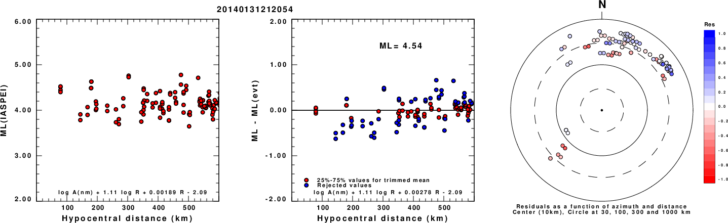
Left: ML computed using the IASPEI formula for Horizontal components. Center: ML residuals computed using a modified IASPEI formula that accounts for path specific attenuation; the values used for the trimmed mean are indicated. The ML relation used for each figure is given at the bottom of each plot. Right: Residuals from new relation as a function of distance and azimuth.

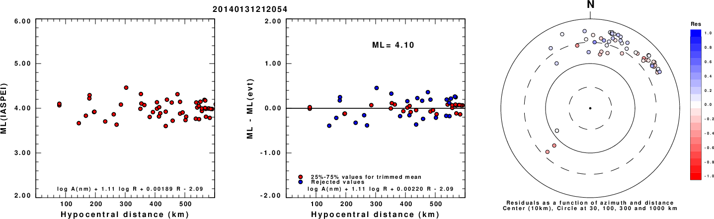
Left: ML computed using the IASPEI formula for Vertical components (research). Center: ML residuals computed using a modified IASPEI formula that accounts for path specific attenuation; the values used for the trimmed mean are indicated. The ML relation used for each figure is given at the bottom of each plot. Right: Residuals from new relation as a function of distance and azimuth.

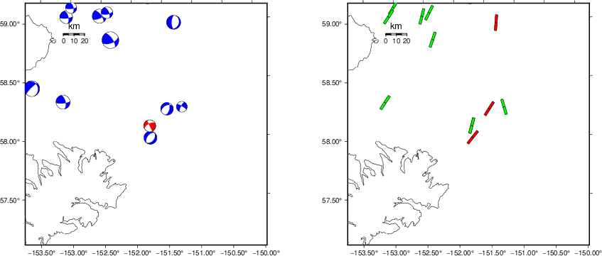
Context

Waveform Inversion using wvfgrd96

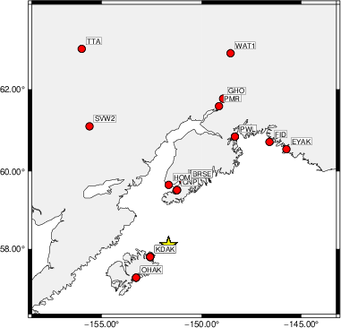
The focal mechanism was determined using broadband seismic waveforms. The location of the event (star) and the stations used for (red) the waveform inversion are shown in the next figure.

Location of broadband stations used for waveform inversion

The program wvfgrd96 was used with good traces observed at short distance to determine the focal mechanism, depth and seismic moment. This technique requires a high quality signal and well determined velocity model for the Green's functions. To the extent that these are the quality data, this type of mechanism should be preferred over the radiation pattern technique which requires the separate step of defining the pressure and tension quadrants and the correct strike.

The observed and predicted traces are filtered using the following gsac commands:

cut a -30 a 180
rtr
taper w 0.1
hp c 0.02 n 3 
lp c 0.06 n 3 

           DEPTH  STK   DIP  RAKE   MW    FIT
WVFGRD96    1.0    20    45   -90   3.59 0.2634
WVFGRD96    3.0   260    55    45   3.65 0.3607
WVFGRD96    5.0    50    55   -10   3.69 0.4145
WVFGRD96    7.0    55    65     0   3.73 0.4676
WVFGRD96    9.0    55    60    -5   3.78 0.4988
WVFGRD96   11.0    55    65    -5   3.81 0.5119
WVFGRD96   13.0   240    65   -15   3.84 0.5363
WVFGRD96   15.0   245    65    -5   3.87 0.5646
WVFGRD96   17.0   245    65     0   3.89 0.5931
WVFGRD96   19.0   245    65     5   3.91 0.6192
WVFGRD96   21.0   245    65     5   3.93 0.6431
WVFGRD96   23.0   245    65     5   3.95 0.6625
WVFGRD96   25.0   245    65     5   3.97 0.6779
WVFGRD96   27.0   245    65     5   3.98 0.6922
WVFGRD96   29.0   245    65     0   4.00 0.7034
WVFGRD96   31.0   245    65     0   4.02 0.7102
WVFGRD96   33.0   245    65     0   4.04 0.7156
WVFGRD96   35.0   245    70    -5   4.07 0.7171
WVFGRD96   37.0   245    70    -5   4.09 0.7199
WVFGRD96   39.0   245    70    -5   4.11 0.7200
WVFGRD96   41.0   245    60     0   4.16 0.7205
WVFGRD96   43.0   245    60     0   4.17 0.7159
WVFGRD96   45.0   245    65    -5   4.20 0.7111
WVFGRD96   47.0   245    65    -5   4.21 0.7026
WVFGRD96   49.0   245    65    -5   4.22 0.6915
WVFGRD96   51.0   245    65    -5   4.23 0.6804
WVFGRD96   53.0   245    65    -5   4.24 0.6679
WVFGRD96   55.0   245    65    -5   4.25 0.6552
WVFGRD96   57.0   245    65    -5   4.26 0.6420
WVFGRD96   59.0   245    65     0   4.25 0.6283
WVFGRD96   61.0   245    65    -5   4.27 0.6154
WVFGRD96   63.0   245    65     0   4.26 0.6023
WVFGRD96   65.0    25    65   -80   4.32 0.5902
WVFGRD96   67.0    30    70   -75   4.31 0.5897
WVFGRD96   69.0    30    70   -75   4.31 0.5889
WVFGRD96   71.0    30    70   -75   4.31 0.5881
WVFGRD96   73.0    30    70   -75   4.31 0.5858
WVFGRD96   75.0    30    70   -75   4.31 0.5829
WVFGRD96   77.0    30    75   -75   4.32 0.5823
WVFGRD96   79.0    30    75   -75   4.32 0.5819
WVFGRD96   81.0    30    75   -75   4.32 0.5788
WVFGRD96   83.0    30    75   -75   4.32 0.5787
WVFGRD96   85.0    30    75   -75   4.32 0.5780
WVFGRD96   87.0    30    75   -75   4.32 0.5748
WVFGRD96   89.0    30    75   -75   4.32 0.5715
WVFGRD96   91.0    30    75   -75   4.32 0.5693
WVFGRD96   93.0    30    75   -70   4.31 0.5683
WVFGRD96   95.0    30    75   -70   4.32 0.5661
WVFGRD96   97.0    30    80   -75   4.33 0.5640
WVFGRD96   99.0    30    80   -75   4.33 0.5636

The best solution is

WVFGRD96   41.0   245    60     0   4.16 0.7205

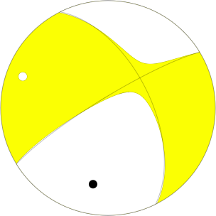
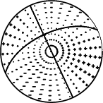
The mechanism corresponding to the best fit is

Figure 1. Waveform inversion focal mechanism

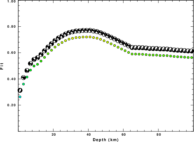
The best fit as a function of depth is given in the following figure:

Figure 2. Depth sensitivity for waveform mechanism

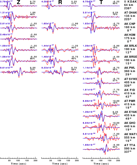
The comparison of the observed and predicted waveforms is given in the next figure. The red traces are the observed and the blue are the predicted. Each observed-predicted component is plotted to the same scale and peak amplitudes are indicated by the numbers to the left of each trace. A pair of numbers is given in black at the right of each predicted traces. The upper number it the time shift required for maximum correlation between the observed and predicted traces. This time shift is required because the synthetics are not computed at exactly the same distance as the observed, the velocity model used in the predictions may not be perfect and the epicentral parameters may be be off. A positive time shift indicates that the prediction is too fast and should be delayed to match the observed trace (shift to the right in this figure). A negative value indicates that the prediction is too slow. The lower number gives the percentage of variance reduction to characterize the individual goodness of fit (100% indicates a perfect fit).

The bandpass filter used in the processing and for the display was

cut a -30 a 180
rtr
taper w 0.1
hp c 0.02 n 3 
lp c 0.06 n 3 

Figure 3. Waveform comparison for selected depth. Red: observed; Blue - predicted. The time shift with respect to the model prediction is indicated. The percent of fit is also indicated. The time scale is relative to the first trace sample.

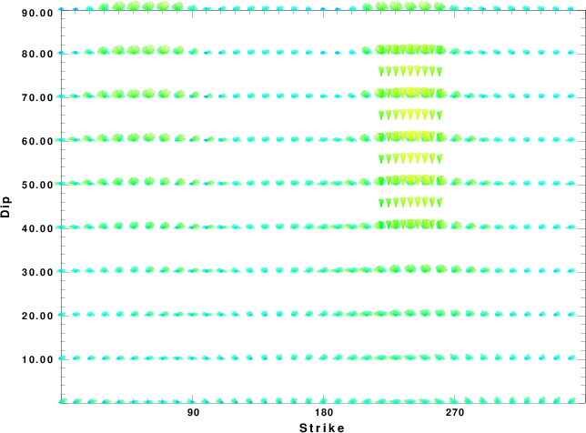
Focal mechanism sensitivity at the preferred depth. The red color indicates a very good fit to the waveforms. Each solution is plotted as a vector at a given value of strike and dip with the angle of the vector representing the rake angle, measured, with respect to the upward vertical (N) in the figure.

A check on the assumed source location is possible by looking at the time shifts between the observed and predicted traces. The time shifts for waveform matching arise for several reasons:

• The origin time and epicentral distance are incorrect
• The velocity model used for the inversion is incorrect
• The velocity model used to define the P-arrival time is not the same as the velocity model used for the waveform inversion (assuming that the initial trace alignment is based on the P arrival time)

 Time_shift = A + B cos Azimuth + C Sin Azimuth

The time shifts for this inversion lead to the next figure:

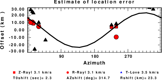
The derived shift in origin time and epicentral coordinates are given at the bottom of the figure.

Velocity Model

The WUS.model used for the waveform synthetic seismograms and for the surface wave eigenfunctions and dispersion is as follows (The format is in the model96 format of Computer Programs in Seismology).

MODEL.01
Model after     8 iterations
ISOTROPIC
KGS
FLAT EARTH
1-D
CONSTANT VELOCITY
LINE08
LINE09
LINE10
LINE11
      H(KM)   VP(KM/S)   VS(KM/S) RHO(GM/CC)         QP         QS       ETAP       ETAS      FREFP      FREFS
     1.9000     3.4065     2.0089     2.2150  0.302E-02  0.679E-02   0.00       0.00       1.00       1.00    
     6.1000     5.5445     3.2953     2.6089  0.349E-02  0.784E-02   0.00       0.00       1.00       1.00    
    13.0000     6.2708     3.7396     2.7812  0.212E-02  0.476E-02   0.00       0.00       1.00       1.00    
    19.0000     6.4075     3.7680     2.8223  0.111E-02  0.249E-02   0.00       0.00       1.00       1.00    
     0.0000     7.9000     4.6200     3.2760  0.164E-10  0.370E-10   0.00       0.00       1.00       1.00