Location
Location ANSS
The ANSS event ID is ak013ctmxi36 and the event page is at
https://earthquake.usgs.gov/earthquakes/eventpage/ak013ctmxi36/executive.
2013/10/06 13:42:17 62.912 -150.573 104.7 4 Alaska
Focal Mechanism
 USGS/SLU Moment Tensor Solution
 ENS  2013/10/06 13:42:17:0  62.91 -150.57 104.7 4.0 Alaska

 Stations used:
   AK.BPAW AK.BWN AK.CCB AK.DHY AK.KTH AK.MCK AK.MLY AK.PPLA
   AK.RND AK.SKN AK.SSN AK.TRF AK.WAT1 AK.WAT2 AK.WAT3 AK.WAT4
   AK.WAT5 AK.WAT6 AK.WAT7 AK.WRH IM.IL31 IU.COLA TA.HDA
   TA.POKR TA.TCOL YE.PIC1 YE.PIC4

 Filtering commands used:
   cut a -30 a 120
   rtr
   taper w 0.1
   hp c 0.02 n 3
   lp c 0.10 n 3

 Best Fitting Double Couple
  Mo = 1.60e+22 dyne-cm
  Mw = 4.07
  Z  = 108 km
  Plane   Strike  Dip  Rake
   NP1      295    60    65
   NP2      158    38   126
  Principal Axes:
   Axis    Value   Plunge  Azimuth
    T   1.60e+22     65     159
    N   0.00e+00     21     308
    P  -1.60e+22     12      43

 Moment Tensor: (dyne-cm)
    Component   Value
       Mxx    -5.84e+21
       Mxy    -8.59e+21
       Mxz    -8.02e+21
       Myy    -6.74e+21
       Myz    -2.39e+14
       Mzz     1.26e+22


                     --------------
                 ##--------------------
              ###----------------------
             ###----------------------- P -
           #####-----------------------   ---
          #########---------------------------
         ------#############-------------------
        ------##################----------------
        ------#####################-------------
       -------########################-----------
       --------#########################---------
       --------###########################-------
       --------#############################-----
        --------#############   #############---
        ---------############ T ##############--
         ---------###########   ###############
          ---------###########################
           ----------########################
             ---------#####################
              -----------#################
                 -----------###########
                     --------------


 Global CMT Convention Moment Tensor:
      R          T          P
  1.26e+22  -8.02e+21   2.39e+14
 -8.02e+21  -5.84e+21   8.59e+21
  2.39e+14   8.59e+21  -6.74e+21


Details of the solution is found at

http://www.eas.slu.edu/eqc/eqc_mt/MECH.NA/20131006134217/index.html
|
Preferred Solution
The preferred solution from an analysis of the surface-wave spectral amplitude radiation pattern, waveform inversion or first motion observations is
      STK = 295
      DIP = 60
     RAKE = 65
       MW = 4.07
       HS = 108.0
The NDK file is 20131006134217.ndk
The waveform inversion is preferred.
Magnitudes
Given the availability of digital waveforms for determination of the moment tensor, this section documents the added processing leading to mLg, if appropriate to the region, and ML by application of the respective IASPEI formulae. As a research study, the linear distance term of the IASPEI formula
for ML is adjusted to remove a linear distance trend in residuals to give a regionally defined ML. The defined ML uses horizontal component recordings, but the same procedure is applied to the vertical components since there may be some interest in vertical component ground motions. Residual plots versus distance may indicate interesting features of ground motion scaling in some distance ranges. A residual plot of the regionalized magnitude is given as a function of distance and azimuth, since data sets may transcend different wave propagation provinces.
ML Magnitude
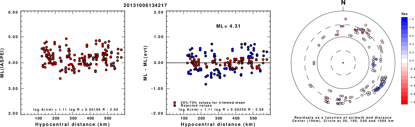
Left: ML computed using the IASPEI formula for Horizontal components. Center: ML residuals computed using a modified IASPEI formula that accounts for path specific attenuation; the values used for the trimmed mean are indicated. The ML relation used for each figure is given at the bottom of each plot.
Right: Residuals from new relation as a function of distance and azimuth.
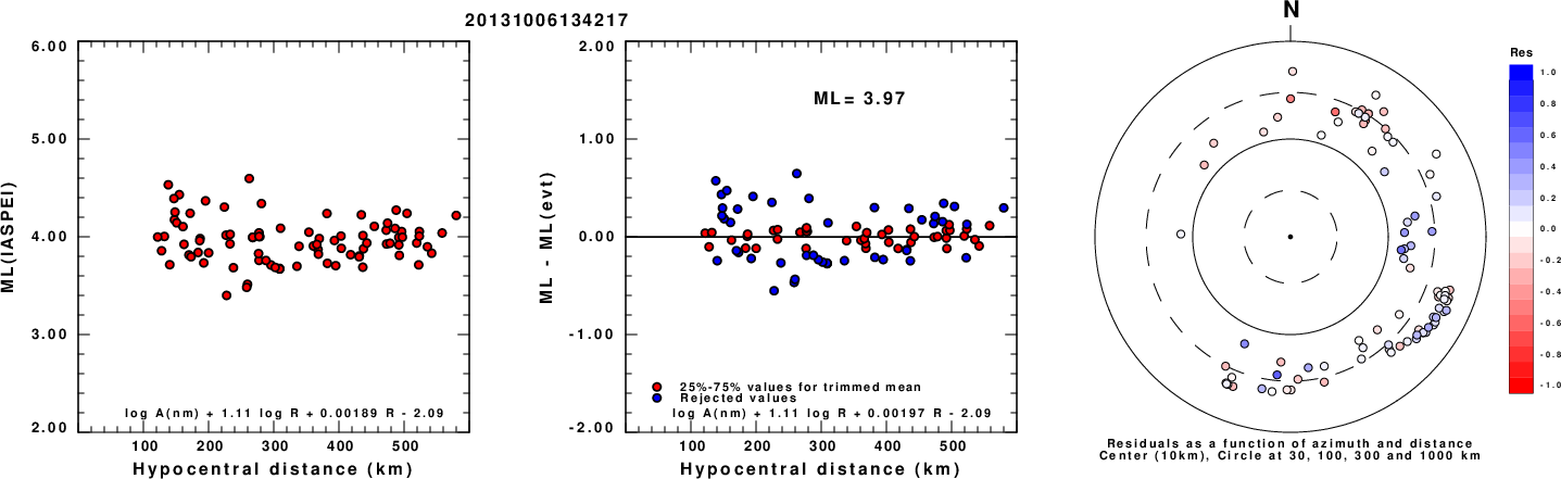
Left: ML computed using the IASPEI formula for Vertical components (research). Center: ML residuals computed using a modified IASPEI formula that accounts for path specific attenuation; the values used for the trimmed mean are indicated. The ML relation used for each figure is given at the bottom of each plot.
Right: Residuals from new relation as a function of distance and azimuth.
Context
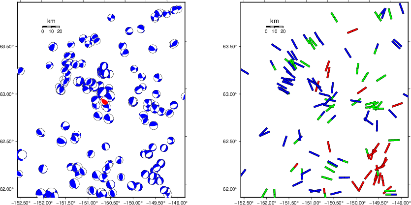
The left panel of the next figure presents the focal mechanism for this earthquake (red) in the context of other nearby events (blue) in the SLU Moment Tensor Catalog. The right panel shows the inferred direction of maximum compressive stress and the type of faulting (green is strike-slip, red is normal, blue is thrust; oblique is shown by a combination of colors). Thus context plot is useful for assessing the appropriateness of the moment tensor of this event.
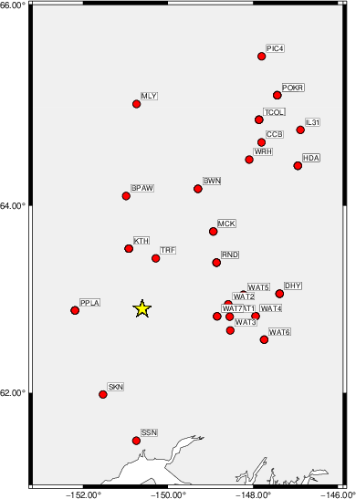
Waveform Inversion using wvfgrd96
The focal mechanism was determined using broadband seismic waveforms. The location of the event (star) and the
stations used for (red) the waveform inversion are shown in the next figure.
|
|
Location of broadband stations used for waveform inversion
|
The program wvfgrd96 was used with good traces observed at short distance to determine the focal mechanism, depth and seismic moment. This technique requires a high quality signal and well determined velocity model for the Green's functions. To the extent that these are the quality data, this type of mechanism should be preferred over the radiation pattern technique which requires the separate step of defining the pressure and tension quadrants and the correct strike.
The observed and predicted traces are filtered using the following gsac commands:
cut a -30 a 120
rtr
taper w 0.1
hp c 0.02 n 3
lp c 0.10 n 3
The results of this grid search are as follow:
           DEPTH  STK   DIP  RAKE   MW    FIT
WVFGRD96    1.0   340    45   -80   3.11 0.1944
WVFGRD96    2.0   330    45   -95   3.26 0.2539
WVFGRD96    3.0   345    40   -75   3.30 0.2036
WVFGRD96    4.0   210    65    30   3.29 0.1968
WVFGRD96    5.0   210    65    35   3.31 0.2177
WVFGRD96    6.0   205    70    35   3.32 0.2344
WVFGRD96    7.0   205    70    40   3.34 0.2518
WVFGRD96    8.0   210    65    45   3.41 0.2555
WVFGRD96    9.0   205    70    45   3.42 0.2677
WVFGRD96   10.0   210    65    50   3.44 0.2764
WVFGRD96   11.0   205    65    50   3.45 0.2823
WVFGRD96   12.0   205    65    50   3.47 0.2854
WVFGRD96   13.0   210    65    55   3.48 0.2864
WVFGRD96   14.0   210    65    55   3.50 0.2857
WVFGRD96   15.0   295    50    35   3.51 0.2857
WVFGRD96   16.0   295    50    35   3.52 0.2866
WVFGRD96   17.0   295    50    40   3.53 0.2871
WVFGRD96   18.0   295    50    40   3.54 0.2863
WVFGRD96   19.0   295    50    35   3.56 0.2845
WVFGRD96   20.0   295    50    40   3.56 0.2821
WVFGRD96   21.0   295    50    40   3.58 0.2785
WVFGRD96   22.0   295    50    35   3.59 0.2753
WVFGRD96   23.0   285    45    25   3.59 0.2717
WVFGRD96   24.0   295    60    35   3.62 0.2684
WVFGRD96   25.0   295    60    40   3.62 0.2661
WVFGRD96   26.0   295    60    40   3.62 0.2624
WVFGRD96   27.0   295    65    40   3.64 0.2608
WVFGRD96   28.0   295    65    40   3.64 0.2602
WVFGRD96   29.0   295    65    40   3.65 0.2594
WVFGRD96   30.0   295    65    40   3.66 0.2593
WVFGRD96   31.0   295    65    40   3.67 0.2586
WVFGRD96   32.0   295    55    30   3.68 0.2642
WVFGRD96   33.0   295    55    30   3.69 0.2706
WVFGRD96   34.0   295    60    30   3.70 0.2767
WVFGRD96   35.0   295    55    35   3.70 0.2819
WVFGRD96   36.0   295    55    35   3.71 0.2856
WVFGRD96   37.0   295    55    35   3.72 0.2880
WVFGRD96   38.0    55    50   -85   3.75 0.2891
WVFGRD96   39.0    55    50   -85   3.77 0.2925
WVFGRD96   40.0    60    50   -85   3.87 0.3008
WVFGRD96   41.0    60    50   -85   3.89 0.3024
WVFGRD96   42.0    60    50   -85   3.90 0.3022
WVFGRD96   43.0   305    45    60   3.86 0.3006
WVFGRD96   44.0    60    50   -85   3.92 0.2984
WVFGRD96   45.0   305    45    55   3.87 0.2976
WVFGRD96   46.0   305    45    55   3.88 0.2986
WVFGRD96   47.0   305    45    55   3.88 0.2979
WVFGRD96   48.0    95    55   -40   3.94 0.3027
WVFGRD96   49.0    95    55   -40   3.95 0.3068
WVFGRD96   50.0    95    55   -40   3.96 0.3108
WVFGRD96   51.0   110    85   -40   3.94 0.3163
WVFGRD96   52.0   110    85   -40   3.94 0.3235
WVFGRD96   53.0   110    85   -40   3.95 0.3310
WVFGRD96   54.0   110    85   -45   3.96 0.3375
WVFGRD96   55.0   305    60    65   3.92 0.3450
WVFGRD96   56.0   305    60    65   3.93 0.3561
WVFGRD96   57.0   305    60    65   3.94 0.3679
WVFGRD96   58.0   305    60    65   3.94 0.3785
WVFGRD96   59.0   305    60    65   3.95 0.3895
WVFGRD96   60.0   305    60    65   3.95 0.4010
WVFGRD96   61.0   305    60    65   3.96 0.4106
WVFGRD96   62.0   305    60    65   3.96 0.4222
WVFGRD96   63.0   305    60    65   3.97 0.4322
WVFGRD96   64.0   305    65    65   3.97 0.4426
WVFGRD96   65.0   305    65    65   3.98 0.4533
WVFGRD96   66.0   305    65    65   3.98 0.4636
WVFGRD96   67.0   300    65    65   3.99 0.4741
WVFGRD96   68.0   300    65    65   3.99 0.4838
WVFGRD96   69.0   300    65    65   4.00 0.4934
WVFGRD96   70.0   300    65    65   4.00 0.5031
WVFGRD96   71.0   300    65    65   4.00 0.5116
WVFGRD96   72.0   300    65    65   4.01 0.5210
WVFGRD96   73.0   300    65    65   4.01 0.5278
WVFGRD96   74.0   300    65    65   4.01 0.5368
WVFGRD96   75.0   300    65    65   4.02 0.5430
WVFGRD96   76.0   300    65    65   4.02 0.5510
WVFGRD96   77.0   300    65    65   4.02 0.5565
WVFGRD96   78.0   300    65    65   4.02 0.5628
WVFGRD96   79.0   300    65    65   4.03 0.5680
WVFGRD96   80.0   300    65    65   4.03 0.5733
WVFGRD96   81.0   300    65    65   4.03 0.5790
WVFGRD96   82.0   300    65    65   4.03 0.5817
WVFGRD96   83.0   300    65    65   4.03 0.5871
WVFGRD96   84.0   300    65    65   4.04 0.5897
WVFGRD96   85.0   300    65    65   4.04 0.5949
WVFGRD96   86.0   300    60    65   4.03 0.5972
WVFGRD96   87.0   300    60    65   4.04 0.6029
WVFGRD96   88.0   300    60    65   4.04 0.6061
WVFGRD96   89.0   300    60    65   4.04 0.6100
WVFGRD96   90.0   300    60    65   4.04 0.6142
WVFGRD96   91.0   300    60    65   4.04 0.6163
WVFGRD96   92.0   300    60    65   4.04 0.6206
WVFGRD96   93.0   300    60    65   4.05 0.6221
WVFGRD96   94.0   300    60    65   4.05 0.6252
WVFGRD96   95.0   300    60    65   4.05 0.6278
WVFGRD96   96.0   300    60    65   4.05 0.6294
WVFGRD96   97.0   300    60    65   4.05 0.6320
WVFGRD96   98.0   300    60    65   4.05 0.6337
WVFGRD96   99.0   300    60    65   4.05 0.6348
WVFGRD96  100.0   300    60    65   4.06 0.6369
WVFGRD96  101.0   300    60    65   4.06 0.6376
WVFGRD96  102.0   300    60    65   4.06 0.6379
WVFGRD96  103.0   300    60    65   4.06 0.6407
WVFGRD96  104.0   300    60    65   4.06 0.6391
WVFGRD96  105.0   300    60    65   4.06 0.6415
WVFGRD96  106.0   295    60    65   4.07 0.6422
WVFGRD96  107.0   295    60    65   4.07 0.6414
WVFGRD96  108.0   295    60    65   4.07 0.6433
WVFGRD96  109.0   295    60    65   4.07 0.6424
WVFGRD96  110.0   295    60    65   4.08 0.6428
WVFGRD96  111.0   295    60    65   4.08 0.6422
WVFGRD96  112.0   295    60    65   4.08 0.6428
WVFGRD96  113.0   295    60    65   4.08 0.6408
WVFGRD96  114.0   295    60    65   4.08 0.6419
WVFGRD96  115.0   295    60    65   4.08 0.6404
WVFGRD96  116.0   295    60    65   4.08 0.6388
WVFGRD96  117.0   295    60    65   4.08 0.6389
WVFGRD96  118.0   295    60    65   4.09 0.6374
WVFGRD96  119.0   295    60    65   4.09 0.6356
WVFGRD96  120.0   295    60    65   4.09 0.6347
WVFGRD96  121.0   295    60    65   4.09 0.6334
WVFGRD96  122.0   295    60    65   4.09 0.6313
WVFGRD96  123.0   295    60    65   4.09 0.6296
WVFGRD96  124.0   295    60    65   4.09 0.6282
WVFGRD96  125.0   295    60    65   4.09 0.6268
WVFGRD96  126.0   295    60    65   4.10 0.6229
WVFGRD96  127.0   295    60    65   4.10 0.6226
WVFGRD96  128.0   295    60    65   4.10 0.6208
WVFGRD96  129.0   295    60    65   4.10 0.6165
The best solution is
WVFGRD96 108.0 295 60 65 4.07 0.6433
The mechanism corresponding to the best fit is
|
|
Figure 1. Waveform inversion focal mechanism
|
The best fit as a function of depth is given in the following figure:
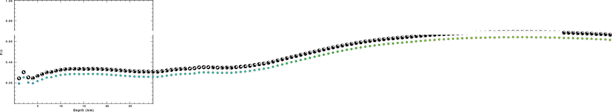
|
|
Figure 2. Depth sensitivity for waveform mechanism
|
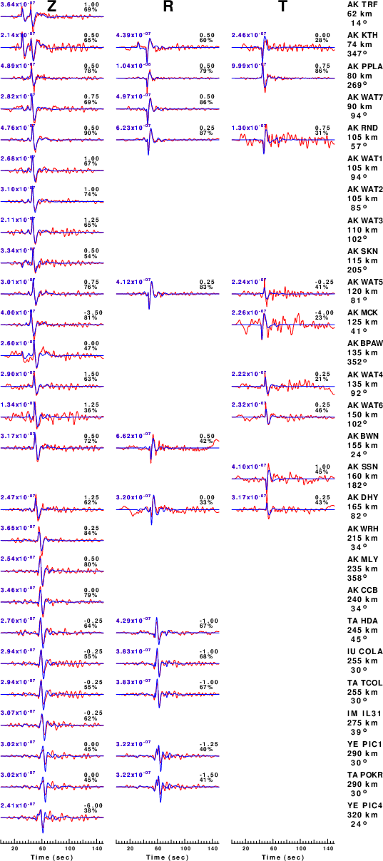
The comparison of the observed and predicted waveforms is given in the next figure. The red traces are the observed and the blue are the predicted.
Each observed-predicted component is plotted to the same scale and peak amplitudes are indicated by the numbers to the left of each trace. A pair of numbers is given in black at the right of each predicted traces. The upper number it the time shift required for maximum correlation between the observed and predicted traces. This time shift is required because the synthetics are not computed at exactly the same distance as the observed, the velocity model used in the predictions may not be perfect and the epicentral parameters may be be off.
A positive time shift indicates that the prediction is too fast and should be delayed to match the observed trace (shift to the right in this figure). A negative value indicates that the prediction is too slow. The lower number gives the percentage of variance reduction to characterize the individual goodness of fit (100% indicates a perfect fit).
The bandpass filter used in the processing and for the display was
cut a -30 a 120
rtr
taper w 0.1
hp c 0.02 n 3
lp c 0.10 n 3
|
|
Figure 3. Waveform comparison for selected depth. Red: observed; Blue - predicted. The time shift with respect to the model prediction is indicated. The percent of fit is also indicated. The time scale is relative to the first trace sample.
|
|
|
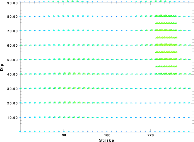
Focal mechanism sensitivity at the preferred depth. The red color indicates a very good fit to the waveforms.
Each solution is plotted as a vector at a given value of strike and dip with the angle of the vector representing the rake angle, measured, with respect to the upward vertical (N) in the figure.
|
A check on the assumed source location is possible by looking at the time shifts between the observed and predicted traces. The time shifts for waveform matching arise for several reasons:
- The origin time and epicentral distance are incorrect
- The velocity model used for the inversion is incorrect
- The velocity model used to define the P-arrival time is not the
same as the velocity model used for the waveform inversion
(assuming that the initial trace alignment is based on the
P arrival time)
Assuming only a mislocation, the time shifts are fit to a functional form:
Time_shift = A + B cos Azimuth + C Sin Azimuth
The time shifts for this inversion lead to the next figure:
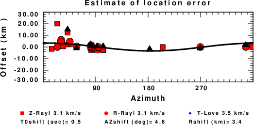
The derived shift in origin time and epicentral coordinates are given at the bottom of the figure.
Velocity Model
The WUS.model used for the waveform synthetic seismograms and for the surface wave eigenfunctions and dispersion is as follows
(The format is in the model96 format of Computer Programs in Seismology).
MODEL.01
Model after     8 iterations
ISOTROPIC
KGS
FLAT EARTH
1-D
CONSTANT VELOCITY
LINE08
LINE09
LINE10
LINE11
      H(KM)   VP(KM/S)   VS(KM/S) RHO(GM/CC)         QP         QS       ETAP       ETAS      FREFP      FREFS
     1.9000     3.4065     2.0089     2.2150  0.302E-02  0.679E-02   0.00       0.00       1.00       1.00
     6.1000     5.5445     3.2953     2.6089  0.349E-02  0.784E-02   0.00       0.00       1.00       1.00
    13.0000     6.2708     3.7396     2.7812  0.212E-02  0.476E-02   0.00       0.00       1.00       1.00
    19.0000     6.4075     3.7680     2.8223  0.111E-02  0.249E-02   0.00       0.00       1.00       1.00
     0.0000     7.9000     4.6200     3.2760  0.164E-10  0.370E-10   0.00       0.00       1.00       1.00
Last Changed Fri Apr 26 09:47:33 PM CDT 2024