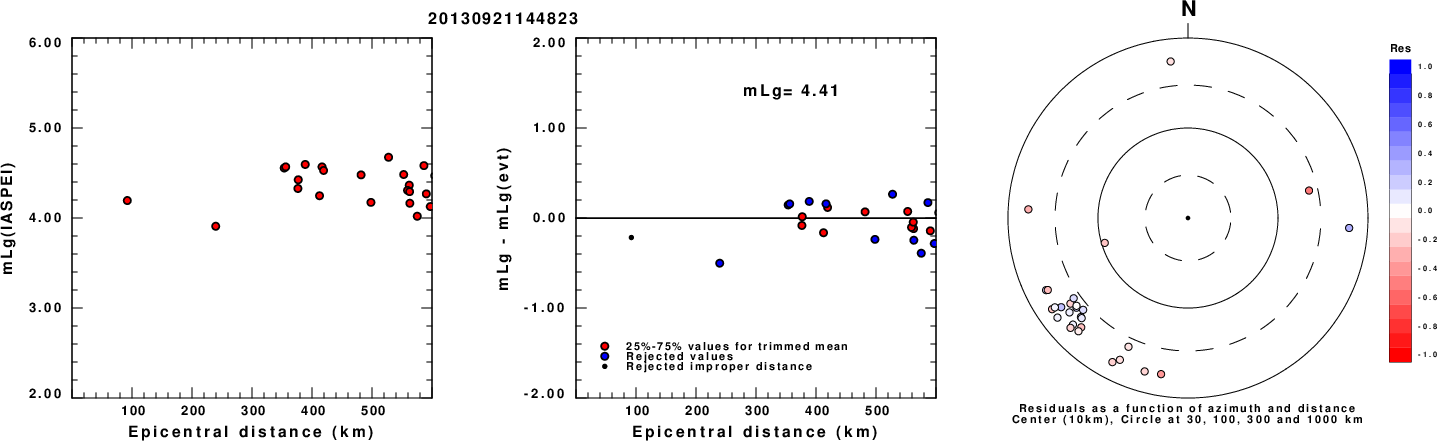
Left: mLg computed using the IASPEI formula. Center: mLg residuals versus epicentral distance ; the values used for the trimmed mean magnitude estimate are indicated. Right: residuals as a function of distance and azimuth.
The ANSS event ID is usb000jx58 and the event page is at https://earthquake.usgs.gov/earthquakes/eventpage/usb000jx58/executive.
2013/09/21 14:48:23 49.767 -65.915 18.0 4.2 Quebec
 USGS/SLU Moment Tensor Solution
 ENS  2013/09/21 14:48:23:0  49.77  -65.92  18.0 4.2 Quebec

 Stations used:
   CN.A11 CN.A16 CN.A21 CN.A54 CN.A61 CN.A64 CN.BATG CN.DMCQ
   CN.DRLN CN.ICQ CN.NATG CN.SCHQ NE.EMMW NE.PQI NE.WVL
   PO.CHGQ PO.LATQ TA.D58A TA.D59A TA.D60A TA.D61A TA.E58A
   TA.E59A TA.E60A TA.E61A TA.F59A TA.F60A TA.F61A TA.H65A

 Filtering commands used:
   cut a -30 a 210
   rtr
   taper w 0.1
   hp c 0.02 n 3
   lp c 0.10 n 3
   br c 0.12 0.25 n 4 p 2

 Best Fitting Double Couple
  Mo = 1.10e+22 dyne-cm
  Mw = 3.96
  Z  = 27 km
  Plane   Strike  Dip  Rake
   NP1      135    50    60
   NP2      357    48   121
  Principal Axes:
   Axis    Value   Plunge  Azimuth
    T   1.10e+22     67     338
    N   0.00e+00     23     155
    P  -1.10e+22      1     246

 Moment Tensor: (dyne-cm)
    Component   Value
       Mxx    -4.76e+20
       Mxy    -4.68e+21
       Mxz     3.66e+21
       Myy    -8.88e+21
       Myz    -1.33e+21
       Mzz     9.35e+21


                     ########------
                 ##############--------
              ###################---------
             #####################---------
           --######################----------
          ---#######################----------
         ----###########   ##########----------
        -----########### T ##########-----------
        ------##########   ###########----------
       -------########################-----------
       --------#######################-----------
       ---------######################-----------
       ----------#####################-----------
        -----------###################----------
           ---------##################----------
         P -----------################---------
           -------------#############---------
           ----------------#########---------
             ------------------####--------
              --------------------########
                 ----------------######
                     ----------####


 Global CMT Convention Moment Tensor:
      R          T          P
  9.35e+21   3.66e+21   1.33e+21
  3.66e+21  -4.76e+20   4.68e+21
  1.33e+21   4.68e+21  -8.88e+21


Details of the solution is found at

http://www.eas.slu.edu/eqc/eqc_mt/MECH.NA/20130921144823/index.html
|
      STK = 135
      DIP = 50
     RAKE = 60
       MW = 3.96
       HS = 27.0
The NDK file is 20130921144823.ndk The waveform inversion is preferred.
Given the availability of digital waveforms for determination of the moment tensor, this section documents the added processing leading to mLg, if appropriate to the region, and ML by application of the respective IASPEI formulae. As a research study, the linear distance term of the IASPEI formula for ML is adjusted to remove a linear distance trend in residuals to give a regionally defined ML. The defined ML uses horizontal component recordings, but the same procedure is applied to the vertical components since there may be some interest in vertical component ground motions. Residual plots versus distance may indicate interesting features of ground motion scaling in some distance ranges. A residual plot of the regionalized magnitude is given as a function of distance and azimuth, since data sets may transcend different wave propagation provinces.
Left: mLg computed using the IASPEI formula. Center: mLg residuals versus epicentral distance ; the values used for the trimmed mean magnitude estimate are indicated.
Right: residuals as a function of distance and azimuth.
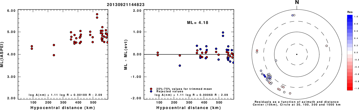
Left: ML computed using the IASPEI formula for Horizontal components. Center: ML residuals computed using a modified IASPEI formula that accounts for path specific attenuation; the values used for the trimmed mean are indicated. The ML relation used for each figure is given at the bottom of each plot.
Right: Residuals from new relation as a function of distance and azimuth.
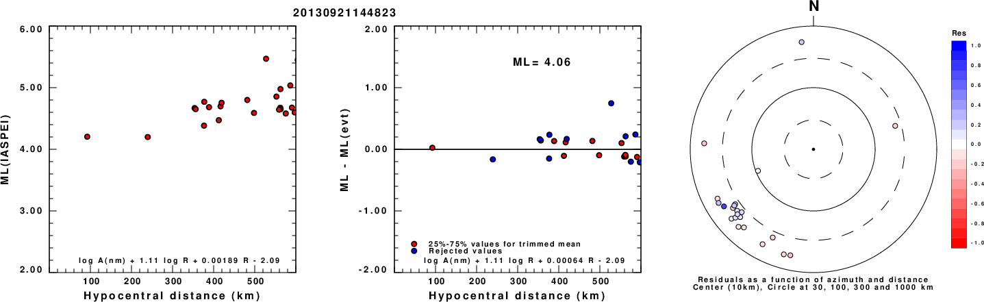
Left: ML computed using the IASPEI formula for Vertical components (research). Center: ML residuals computed using a modified IASPEI formula that accounts for path specific attenuation; the values used for the trimmed mean are indicated. The ML relation used for each figure is given at the bottom of each plot.
Right: Residuals from new relation as a function of distance and azimuth.
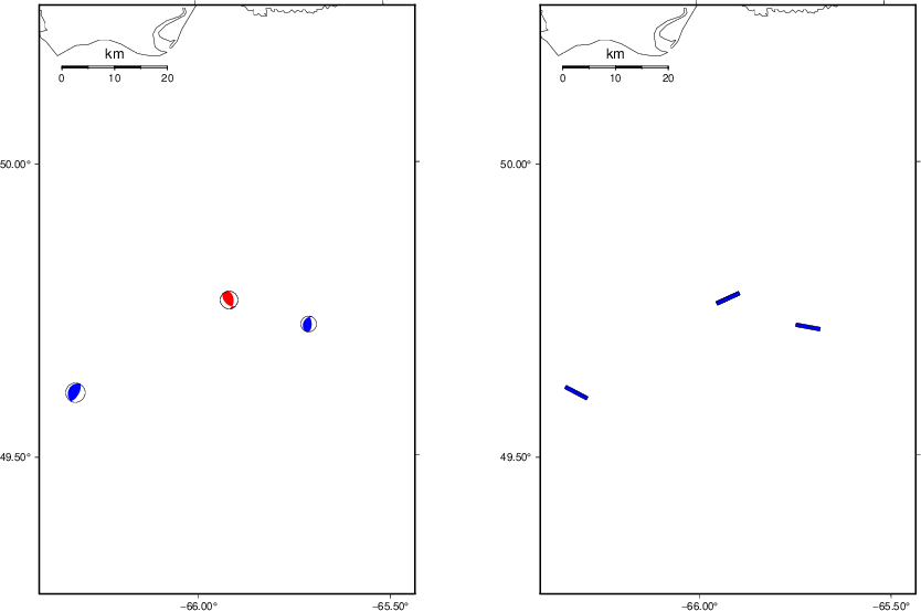 |
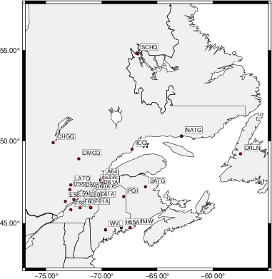
The focal mechanism was determined using broadband seismic waveforms. The location of the event (star) and the stations used for (red) the waveform inversion are shown in the next figure.
|
|
|
The program wvfgrd96 was used with good traces observed at short distance to determine the focal mechanism, depth and seismic moment. This technique requires a high quality signal and well determined velocity model for the Green's functions. To the extent that these are the quality data, this type of mechanism should be preferred over the radiation pattern technique which requires the separate step of defining the pressure and tension quadrants and the correct strike.
The observed and predicted traces are filtered using the following gsac commands:
cut a -30 a 210
rtr
taper w 0.1
hp c 0.02 n 3
lp c 0.10 n 3
br c 0.12 0.25 n 4 p 2
The results of this grid search are as follow:
           DEPTH  STK   DIP  RAKE   MW    FIT
WVFGRD96    0.5   300    45   -95   3.64 0.5769
WVFGRD96    1.0   305    45   -90   3.68 0.5995
WVFGRD96    2.0   325    45   -90   3.75 0.6009
WVFGRD96    3.0   190    65   -30   3.83 0.5238
WVFGRD96    4.0    20    65     5   3.85 0.4751
WVFGRD96    5.0   200    30   -10   3.77 0.5010
WVFGRD96    6.0   205    30    -5   3.75 0.5296
WVFGRD96    7.0   210    30     0   3.74 0.5516
WVFGRD96    8.0   210    45    20   3.80 0.5685
WVFGRD96    9.0   210    45    20   3.79 0.5827
WVFGRD96   10.0   215    35    15   3.78 0.5913
WVFGRD96   11.0   210    45    20   3.82 0.6031
WVFGRD96   12.0   210    45    20   3.83 0.6138
WVFGRD96   13.0   215    45    30   3.84 0.6240
WVFGRD96   14.0   215    45    30   3.85 0.6332
WVFGRD96   15.0   215    45    30   3.85 0.6411
WVFGRD96   16.0   215    45    30   3.86 0.6480
WVFGRD96   17.0   220    40    25   3.84 0.6543
WVFGRD96   18.0   210    50    30   3.89 0.6597
WVFGRD96   19.0   210    50    30   3.90 0.6644
WVFGRD96   20.0   220    35    20   3.88 0.6658
WVFGRD96   21.0   225    30    20   3.87 0.6684
WVFGRD96   22.0   135    60    60   3.91 0.6764
WVFGRD96   23.0   140    55    60   3.92 0.6841
WVFGRD96   24.0   135    55    55   3.94 0.6900
WVFGRD96   25.0   135    55    55   3.95 0.6944
WVFGRD96   26.0   130    55    55   3.96 0.6962
WVFGRD96   27.0   135    50    60   3.96 0.6964
WVFGRD96   28.0   135    50    60   3.97 0.6954
WVFGRD96   29.0   135    50    60   3.98 0.6921
WVFGRD96   30.0   130    50    55   4.00 0.6882
WVFGRD96   31.0   130    50    55   4.01 0.6821
WVFGRD96   32.0   130    50    55   4.03 0.6738
WVFGRD96   33.0   135    45    60   4.03 0.6650
WVFGRD96   34.0   135    45    60   4.04 0.6543
WVFGRD96   35.0   135    45    60   4.05 0.6417
WVFGRD96   36.0   135    45    55   4.08 0.6283
WVFGRD96   37.0   130    45    55   4.09 0.6122
WVFGRD96   38.0   130    45    55   4.11 0.5947
WVFGRD96   39.0   145    40    60   4.12 0.5750
WVFGRD96   40.0   305    70   -70   4.16 0.5656
WVFGRD96   41.0   305    70   -70   4.17 0.5488
WVFGRD96   42.0   310    70   -65   4.17 0.5340
WVFGRD96   43.0   310    70   -65   4.17 0.5206
WVFGRD96   44.0   310    70   -60   4.18 0.5080
WVFGRD96   45.0   310    70   -60   4.18 0.4821
WVFGRD96   46.0   310    70   -60   4.18 0.4709
WVFGRD96   47.0   310    70   -55   4.20 0.4601
WVFGRD96   48.0   310    70   -55   4.20 0.4500
WVFGRD96   49.0   310    70   -55   4.21 0.4401
WVFGRD96   50.0   310    70   -55   4.21 0.4304
The best solution is
WVFGRD96 27.0 135 50 60 3.96 0.6964
The mechanism corresponding to the best fit is
|
|
|
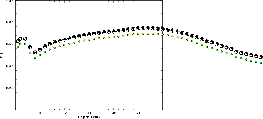
The best fit as a function of depth is given in the following figure:
|
|
|
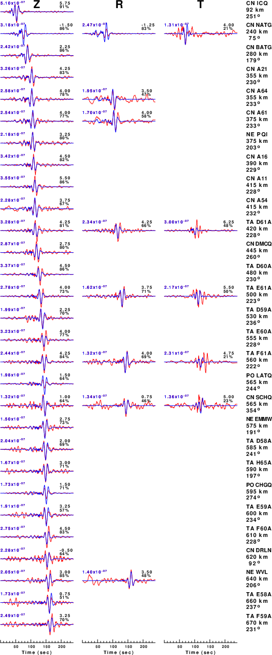
The comparison of the observed and predicted waveforms is given in the next figure. The red traces are the observed and the blue are the predicted. Each observed-predicted component is plotted to the same scale and peak amplitudes are indicated by the numbers to the left of each trace. A pair of numbers is given in black at the right of each predicted traces. The upper number it the time shift required for maximum correlation between the observed and predicted traces. This time shift is required because the synthetics are not computed at exactly the same distance as the observed, the velocity model used in the predictions may not be perfect and the epicentral parameters may be be off. A positive time shift indicates that the prediction is too fast and should be delayed to match the observed trace (shift to the right in this figure). A negative value indicates that the prediction is too slow. The lower number gives the percentage of variance reduction to characterize the individual goodness of fit (100% indicates a perfect fit).
The bandpass filter used in the processing and for the display was
cut a -30 a 210
rtr
taper w 0.1
hp c 0.02 n 3
lp c 0.10 n 3
br c 0.12 0.25 n 4 p 2
|
| Figure 3. Waveform comparison for selected depth. Red: observed; Blue - predicted. The time shift with respect to the model prediction is indicated. The percent of fit is also indicated. The time scale is relative to the first trace sample. |
|
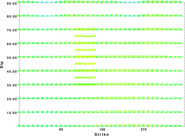
| Focal mechanism sensitivity at the preferred depth. The red color indicates a very good fit to the waveforms. Each solution is plotted as a vector at a given value of strike and dip with the angle of the vector representing the rake angle, measured, with respect to the upward vertical (N) in the figure. |
A check on the assumed source location is possible by looking at the time shifts between the observed and predicted traces. The time shifts for waveform matching arise for several reasons:
Time_shift = A + B cos Azimuth + C Sin Azimuth
The time shifts for this inversion lead to the next figure:
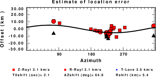
The derived shift in origin time and epicentral coordinates are given at the bottom of the figure.
The CUS.model used for the waveform synthetic seismograms and for the surface wave eigenfunctions and dispersion is as follows (The format is in the model96 format of Computer Programs in Seismology).
MODEL.01
CUS Model with Q from simple gamma values
ISOTROPIC
KGS
FLAT EARTH
1-D
CONSTANT VELOCITY
LINE08
LINE09
LINE10
LINE11
  H(KM) VP(KM/S) VS(KM/S) RHO(GM/CC)   QP   QS  ETAP  ETAS  FREFP  FREFS
  1.0000  5.0000  2.8900  2.5000 0.172E-02 0.387E-02 0.00  0.00  1.00  1.00
  9.0000  6.1000  3.5200  2.7300 0.160E-02 0.363E-02 0.00  0.00  1.00  1.00
 10.0000  6.4000  3.7000  2.8200 0.149E-02 0.336E-02 0.00  0.00  1.00  1.00
 20.0000  6.7000  3.8700  2.9020 0.000E-04 0.000E-04 0.00  0.00  1.00  1.00
  0.0000  8.1500  4.7000  3.3640 0.194E-02 0.431E-02 0.00  0.00  1.00  1.00