Location
SLU Location
To check the ANSS location or to compare the observed P-wave first motions to the moment tensor solution, P- and S-wave first arrival times were manually read together with the P-wave first motions. The subsequent output of the program elocate is given in the file elocate.txt. The first motion plot is shown below.
Location ANSS
The ANSS event ID is usb000jx4l and the event page is at
https://earthquake.usgs.gov/earthquakes/eventpage/usb000jx4l/executive.
2013/09/21 13:16:31 42.974 -109.128 76.2 4.8 Wyoming
Focal Mechanism
 USGS/SLU Moment Tensor Solution
 ENS  2013/09/21 13:16:31:0  42.97 -109.13  76.2 4.8 Wyoming

 Stations used:
   IU.RSSD IW.DLMT IW.FLWY IW.FXWY IW.IMW IW.LOHW IW.MOOW
   IW.REDW IW.RWWY IW.SNOW IW.TPAW TA.H17A TA.Q24A US.AHID
   US.BOZ US.LKWY US.MSO US.RLMT WY.YHB WY.YHH WY.YHL WY.YMP
   WY.YNE WY.YNR WY.YTP

 Filtering commands used:
   cut a -30 a 180
   rtr
   taper w 0.1
   hp c 0.02 n 3
   lp c 0.08 n 3

 Best Fitting Double Couple
  Mo = 1.80e+23 dyne-cm
  Mw = 4.77
  Z  = 76 km
  Plane   Strike  Dip  Rake
   NP1       65    65    30
   NP2      321    63   152
  Principal Axes:
   Axis    Value   Plunge  Azimuth
    T   1.80e+23     38     284
    N   0.00e+00     52     101
    P  -1.80e+23      1     193

 Moment Tensor: (dyne-cm)
    Component   Value
       Mxx    -1.65e+23
       Mxy    -6.44e+22
       Mxz     2.46e+22
       Myy     9.59e+22
       Myz    -8.41e+22
       Mzz     6.89e+22


                     --------------
                 ----------------------
              ####------------------------
             #########---------------------
           ##############--------------------
          ##################------------------
         #####################-----------------
        #######################---------------##
        ######   ################-----------####
       ####### T #################---------######
       #######   ###################-----########
       ##############################--##########
       #############################--###########
        #########################------#########
        #####################-----------########
         ###############----------------#######
          -------------------------------#####
           ------------------------------####
             ----------------------------##
              ---------------------------#
                 -----   --------------
                     - P ----------


 Global CMT Convention Moment Tensor:
      R          T          P
  6.89e+22   2.46e+22   8.41e+22
  2.46e+22  -1.65e+23   6.44e+22
  8.41e+22   6.44e+22   9.59e+22


Details of the solution is found at

http://www.eas.slu.edu/eqc/eqc_mt/MECH.NA/20130921131631/index.html
|
Preferred Solution
The preferred solution from an analysis of the surface-wave spectral amplitude radiation pattern, waveform inversion or first motion observations is
      STK = 65
      DIP = 65
     RAKE = 30
       MW = 4.77
       HS = 76.0
The NDK file is 20130921131631.ndk
The waveform inversion is preferred.
Moment Tensor Comparison
The following compares this source inversion to those provided by others. The purpose is to look for major differences and also to note slight differences that might be inherent to the processing procedure. For completeness the USGS/SLU solution is repeated from above.
| SLU |
USGSMT |
GCMT |
SLUFM |
 USGS/SLU Moment Tensor Solution
 ENS  2013/09/21 13:16:31:0  42.97 -109.13  76.2 4.8 Wyoming

 Stations used:
   IU.RSSD IW.DLMT IW.FLWY IW.FXWY IW.IMW IW.LOHW IW.MOOW
   IW.REDW IW.RWWY IW.SNOW IW.TPAW TA.H17A TA.Q24A US.AHID
   US.BOZ US.LKWY US.MSO US.RLMT WY.YHB WY.YHH WY.YHL WY.YMP
   WY.YNE WY.YNR WY.YTP

 Filtering commands used:
   cut a -30 a 180
   rtr
   taper w 0.1
   hp c 0.02 n 3
   lp c 0.08 n 3

 Best Fitting Double Couple
  Mo = 1.80e+23 dyne-cm
  Mw = 4.77
  Z  = 76 km
  Plane   Strike  Dip  Rake
   NP1       65    65    30
   NP2      321    63   152
  Principal Axes:
   Axis    Value   Plunge  Azimuth
    T   1.80e+23     38     284
    N   0.00e+00     52     101
    P  -1.80e+23      1     193

 Moment Tensor: (dyne-cm)
    Component   Value
       Mxx    -1.65e+23
       Mxy    -6.44e+22
       Mxz     2.46e+22
       Myy     9.59e+22
       Myz    -8.41e+22
       Mzz     6.89e+22


                     --------------
                 ----------------------
              ####------------------------
             #########---------------------
           ##############--------------------
          ##################------------------
         #####################-----------------
        #######################---------------##
        ######   ################-----------####
       ####### T #################---------######
       #######   ###################-----########
       ##############################--##########
       #############################--###########
        #########################------#########
        #####################-----------########
         ###############----------------#######
          -------------------------------#####
           ------------------------------####
             ----------------------------##
              ---------------------------#
                 -----   --------------
                     - P ----------


 Global CMT Convention Moment Tensor:
      R          T          P
  6.89e+22   2.46e+22   8.41e+22
  2.46e+22  -1.65e+23   6.44e+22
  8.41e+22   6.44e+22   9.59e+22


Details of the solution is found at

http://www.eas.slu.edu/eqc/eqc_mt/MECH.NA/20130921131631/index.html
|
Regional Moment Tensor (Mwr)

Moment
    2.71e+16 N-m
Magnitude
    4.9
Percent DC
    45%
Depth
    78.0 km
Updated
    2013-09-21 15:44:17 UTC
Author
    us
Catalog
    us
Contributor
    us
Code
    us_b000jx4l_mwr

Principal Axes
Axis	Value	Plunge	Azimuth
T	2.331	52	296
N	0.641	38	103
P	-2.971	6	198
Nodal Planes
Plane	Strike	Dip	Rake
NP1	78°	61	46
NP2	322°	51	142

|
September 21, 2013, WYOMING, MW=4.8

Meredith Nettles
Goran Ekstrom

CENTROID-MOMENT-TENSOR  SOLUTION
GCMT EVENT:     S201309211316A
DATA: IU II LD DK G  TA US BK CI
SURFACE WAVES: 101S, 160C, T= 50
TIMESTAMP:      Q-20130921162219
CENTROID LOCATION:
ORIGIN TIME:      13:16:35.5 0.2
LAT:42.99N 0.02;LON:109.12W 0.02
DEP: 82.0  3.6;TRIANG HDUR:  0.6
MOMENT TENSOR: SCALE 10**23 D-CM
RR= 0.445 0.072; TT=-2.090 0.070
PP= 1.640 0.069; RT= 0.247 0.043
RP= 0.786 0.031; TP= 0.631 0.073
PRINCIPAL AXES:
1.(T) VAL=  2.138;PLG=26;AZM=280
2.(N)       0.057;    64;     93
3.(P)      -2.199;     3;    189
BEST DBLE.COUPLE:M0= 2.17*10**23
NP1: STRIKE=321;DIP=70;SLIP= 163
NP2: STRIKE= 57;DIP=74;SLIP=  21

            -----------
        -------------------
      ####-------------------
    #########------------------
   ############----------------#
  ###############-------------###
  ##   ############---------#####
 ### T #############------########
 ###   ###############--##########
 #####################-###########
 ##################-----##########
  ##############---------########
  ##########--------------#######
   ####--------------------#####
    -----------------------####
      ----------------------#
        ------   ----------
            -- P ------
|
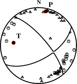
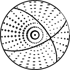
First motions and takeoff angles from an elocate run.
|
Magnitudes
Given the availability of digital waveforms for determination of the moment tensor, this section documents the added processing leading to mLg, if appropriate to the region, and ML by application of the respective IASPEI formulae. As a research study, the linear distance term of the IASPEI formula
for ML is adjusted to remove a linear distance trend in residuals to give a regionally defined ML. The defined ML uses horizontal component recordings, but the same procedure is applied to the vertical components since there may be some interest in vertical component ground motions. Residual plots versus distance may indicate interesting features of ground motion scaling in some distance ranges. A residual plot of the regionalized magnitude is given as a function of distance and azimuth, since data sets may transcend different wave propagation provinces.
ML Magnitude
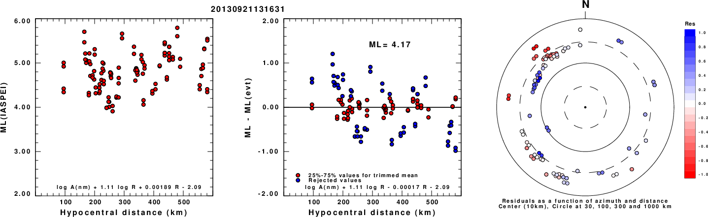
Left: ML computed using the IASPEI formula for Horizontal components. Center: ML residuals computed using a modified IASPEI formula that accounts for path specific attenuation; the values used for the trimmed mean are indicated. The ML relation used for each figure is given at the bottom of each plot.
Right: Residuals from new relation as a function of distance and azimuth.
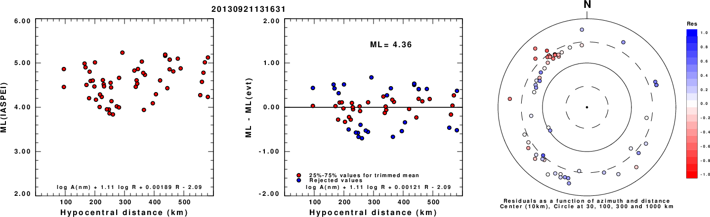
Left: ML computed using the IASPEI formula for Vertical components (research). Center: ML residuals computed using a modified IASPEI formula that accounts for path specific attenuation; the values used for the trimmed mean are indicated. The ML relation used for each figure is given at the bottom of each plot.
Right: Residuals from new relation as a function of distance and azimuth.
Context
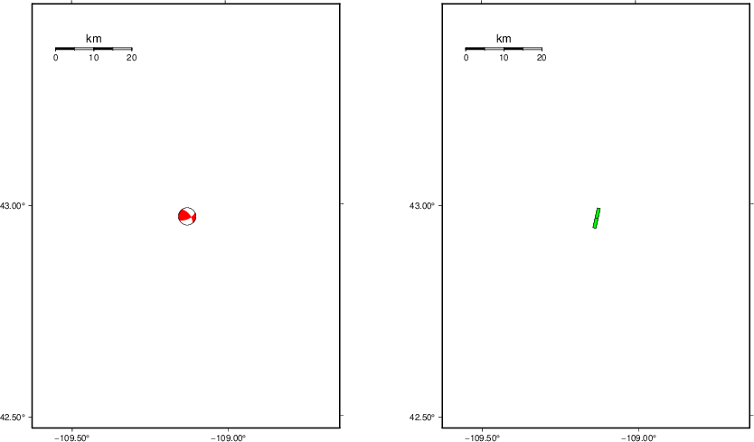
The left panel of the next figure presents the focal mechanism for this earthquake (red) in the context of other nearby events (blue) in the SLU Moment Tensor Catalog. The right panel shows the inferred direction of maximum compressive stress and the type of faulting (green is strike-slip, red is normal, blue is thrust; oblique is shown by a combination of colors). Thus context plot is useful for assessing the appropriateness of the moment tensor of this event.
Waveform Inversion using wvfgrd96
The focal mechanism was determined using broadband seismic waveforms. The location of the event (star) and the
stations used for (red) the waveform inversion are shown in the next figure.

|
|
Location of broadband stations used for waveform inversion
|
The program wvfgrd96 was used with good traces observed at short distance to determine the focal mechanism, depth and seismic moment. This technique requires a high quality signal and well determined velocity model for the Green's functions. To the extent that these are the quality data, this type of mechanism should be preferred over the radiation pattern technique which requires the separate step of defining the pressure and tension quadrants and the correct strike.
The observed and predicted traces are filtered using the following gsac commands:
cut a -30 a 180
rtr
taper w 0.1
hp c 0.02 n 3
lp c 0.08 n 3
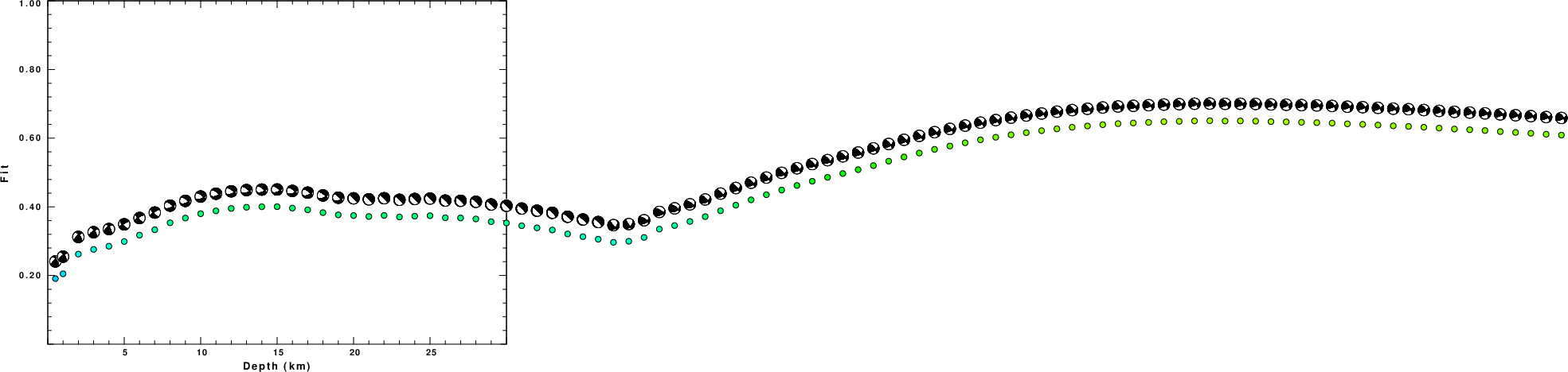
The results of this grid search are as follow:
           DEPTH  STK   DIP  RAKE   MW    FIT
WVFGRD96    0.5   330    60    30   3.69 0.1911
WVFGRD96    1.0   330    60    20   3.72 0.2050
WVFGRD96    2.0   330    60    25   3.83 0.2624
WVFGRD96    3.0   330    65    20   3.87 0.2761
WVFGRD96    4.0   335    70    40   3.93 0.2853
WVFGRD96    5.0   140    65   -15   3.93 0.2991
WVFGRD96    6.0   140    70   -20   3.95 0.3175
WVFGRD96    7.0   140    70   -15   3.98 0.3333
WVFGRD96    8.0   310    60   -40   4.06 0.3536
WVFGRD96    9.0   310    60   -45   4.10 0.3674
WVFGRD96   10.0   310    60   -45   4.11 0.3800
WVFGRD96   11.0   310    60   -45   4.13 0.3883
WVFGRD96   12.0   310    65   -45   4.15 0.3953
WVFGRD96   13.0   310    65   -45   4.16 0.3988
WVFGRD96   14.0   310    65   -45   4.17 0.4003
WVFGRD96   15.0   310    65   -45   4.19 0.4005
WVFGRD96   16.0   310    65   -45   4.20 0.3963
WVFGRD96   17.0   310    65   -45   4.21 0.3913
WVFGRD96   18.0   310    65   -45   4.22 0.3832
WVFGRD96   19.0   315    70   -50   4.24 0.3767
WVFGRD96   20.0   180     5   -45   4.31 0.3748
WVFGRD96   21.0   180     5   -45   4.33 0.3719
WVFGRD96   22.0   170     5   -55   4.34 0.3750
WVFGRD96   23.0   190    10   -35   4.35 0.3705
WVFGRD96   24.0   185    10   -40   4.36 0.3729
WVFGRD96   25.0   190    10   -35   4.37 0.3742
WVFGRD96   26.0   180    10   -45   4.38 0.3682
WVFGRD96   27.0   180    10   -45   4.39 0.3677
WVFGRD96   28.0   180    10   -45   4.40 0.3647
WVFGRD96   29.0   175    10   -50   4.41 0.3568
WVFGRD96   30.0   175    10   -50   4.42 0.3530
WVFGRD96   31.0   175    10   -50   4.43 0.3450
WVFGRD96   32.0   175    10   -50   4.43 0.3388
WVFGRD96   33.0   175    10   -50   4.44 0.3326
WVFGRD96   34.0   165    10   -55   4.45 0.3212
WVFGRD96   35.0   170    10   -50   4.46 0.3131
WVFGRD96   36.0   175    10   -50   4.44 0.3057
WVFGRD96   37.0    40    40   -15   4.39 0.2968
WVFGRD96   38.0    45    45   -15   4.39 0.2998
WVFGRD96   39.0    60    45    35   4.42 0.3109
WVFGRD96   40.0    70    40    45   4.54 0.3352
WVFGRD96   41.0    65    45    40   4.55 0.3456
WVFGRD96   42.0    70    40    40   4.58 0.3574
WVFGRD96   43.0    60    45    20   4.57 0.3715
WVFGRD96   44.0    60    45    20   4.59 0.3886
WVFGRD96   45.0    60    50    20   4.59 0.4049
WVFGRD96   46.0    60    50    20   4.61 0.4204
WVFGRD96   47.0    60    50    20   4.62 0.4352
WVFGRD96   48.0    65    50    25   4.64 0.4490
WVFGRD96   49.0    65    50    25   4.65 0.4623
WVFGRD96   50.0    65    50    25   4.66 0.4746
WVFGRD96   51.0    65    50    25   4.67 0.4860
WVFGRD96   52.0    65    50    30   4.69 0.4971
WVFGRD96   53.0    65    50    30   4.70 0.5083
WVFGRD96   54.0    60    55    20   4.68 0.5202
WVFGRD96   55.0    60    55    20   4.69 0.5331
WVFGRD96   56.0    60    55    20   4.70 0.5453
WVFGRD96   57.0    60    55    20   4.71 0.5567
WVFGRD96   58.0    60    60    20   4.70 0.5675
WVFGRD96   59.0    60    60    20   4.71 0.5771
WVFGRD96   60.0    60    60    20   4.72 0.5866
WVFGRD96   61.0    60    60    20   4.72 0.5952
WVFGRD96   62.0    60    60    20   4.73 0.6027
WVFGRD96   63.0    60    60    20   4.73 0.6098
WVFGRD96   64.0    60    65    25   4.73 0.6161
WVFGRD96   65.0    60    65    25   4.73 0.6218
WVFGRD96   66.0    65    60    25   4.75 0.6272
WVFGRD96   67.0    65    60    25   4.76 0.6318
WVFGRD96   68.0    65    60    25   4.76 0.6356
WVFGRD96   69.0    65    60    25   4.76 0.6393
WVFGRD96   70.0    65    60    25   4.77 0.6423
WVFGRD96   71.0    65    60    25   4.77 0.6442
WVFGRD96   72.0    65    65    30   4.76 0.6460
WVFGRD96   73.0    65    65    30   4.77 0.6479
WVFGRD96   74.0    65    65    30   4.77 0.6490
WVFGRD96   75.0    65    65    30   4.77 0.6503
WVFGRD96   76.0    65    65    30   4.77 0.6508
WVFGRD96   77.0    65    65    30   4.77 0.6500
WVFGRD96   78.0    65    65    30   4.78 0.6502
WVFGRD96   79.0    65    65    30   4.78 0.6497
WVFGRD96   80.0    65    65    30   4.78 0.6482
WVFGRD96   81.0    65    70    30   4.77 0.6474
WVFGRD96   82.0    65    70    30   4.77 0.6463
WVFGRD96   83.0    65    70    30   4.77 0.6453
WVFGRD96   84.0    65    70    30   4.77 0.6439
WVFGRD96   85.0    65    70    30   4.77 0.6417
WVFGRD96   86.0    65    70    30   4.77 0.6403
WVFGRD96   87.0    65    70    30   4.77 0.6383
WVFGRD96   88.0    65    70    30   4.77 0.6359
WVFGRD96   89.0    65    70    30   4.77 0.6343
WVFGRD96   90.0    65    70    30   4.77 0.6319
WVFGRD96   91.0    65    70    30   4.77 0.6294
WVFGRD96   92.0    65    70    30   4.78 0.6267
WVFGRD96   93.0    65    70    30   4.78 0.6246
WVFGRD96   94.0    65    70    30   4.78 0.6222
WVFGRD96   95.0    65    70    30   4.78 0.6193
WVFGRD96   96.0    65    70    30   4.78 0.6168
WVFGRD96   97.0    65    70    30   4.78 0.6142
WVFGRD96   98.0    65    70    30   4.78 0.6115
WVFGRD96   99.0    65    70    30   4.78 0.6089
The best solution is
WVFGRD96 76.0 65 65 30 4.77 0.6508
The mechanism corresponding to the best fit is
|
|
Figure 1. Waveform inversion focal mechanism
|
The best fit as a function of depth is given in the following figure:
|
|
Figure 2. Depth sensitivity for waveform mechanism
|
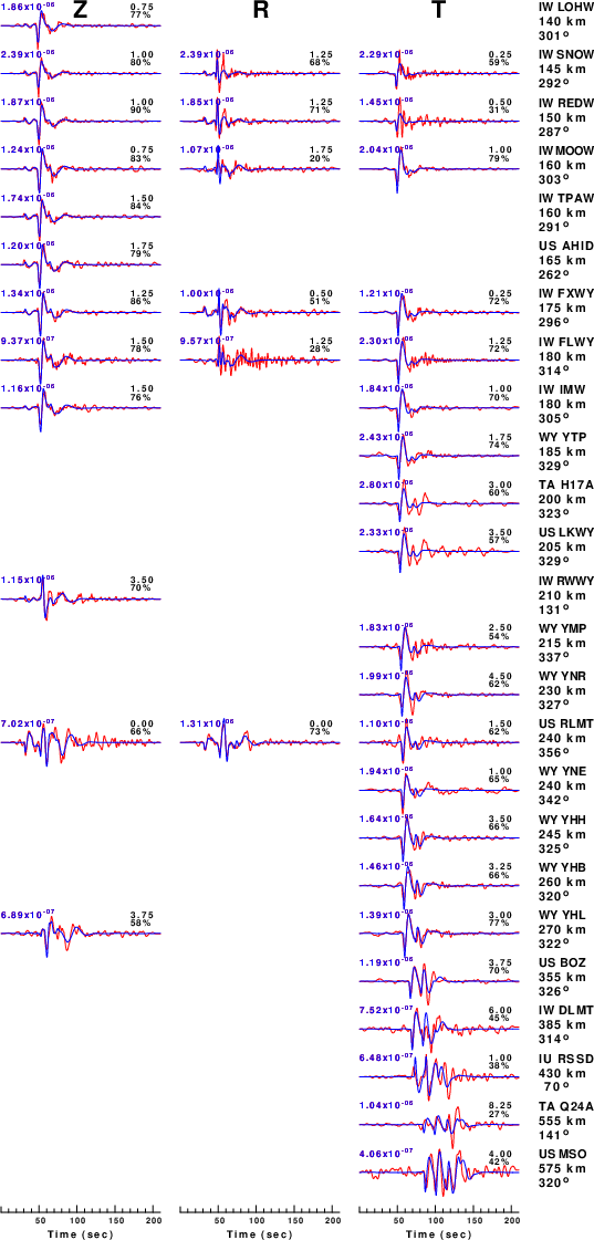
The comparison of the observed and predicted waveforms is given in the next figure. The red traces are the observed and the blue are the predicted.
Each observed-predicted component is plotted to the same scale and peak amplitudes are indicated by the numbers to the left of each trace. A pair of numbers is given in black at the right of each predicted traces. The upper number it the time shift required for maximum correlation between the observed and predicted traces. This time shift is required because the synthetics are not computed at exactly the same distance as the observed, the velocity model used in the predictions may not be perfect and the epicentral parameters may be be off.
A positive time shift indicates that the prediction is too fast and should be delayed to match the observed trace (shift to the right in this figure). A negative value indicates that the prediction is too slow. The lower number gives the percentage of variance reduction to characterize the individual goodness of fit (100% indicates a perfect fit).
The bandpass filter used in the processing and for the display was
cut a -30 a 180
rtr
taper w 0.1
hp c 0.02 n 3
lp c 0.08 n 3
|
|
Figure 3. Waveform comparison for selected depth. Red: observed; Blue - predicted. The time shift with respect to the model prediction is indicated. The percent of fit is also indicated. The time scale is relative to the first trace sample.
|
|
|
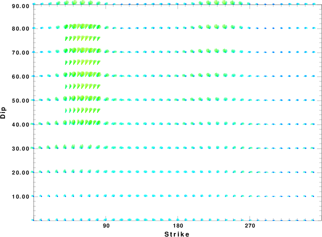
Focal mechanism sensitivity at the preferred depth. The red color indicates a very good fit to the waveforms.
Each solution is plotted as a vector at a given value of strike and dip with the angle of the vector representing the rake angle, measured, with respect to the upward vertical (N) in the figure.
|
A check on the assumed source location is possible by looking at the time shifts between the observed and predicted traces. The time shifts for waveform matching arise for several reasons:
- The origin time and epicentral distance are incorrect
- The velocity model used for the inversion is incorrect
- The velocity model used to define the P-arrival time is not the
same as the velocity model used for the waveform inversion
(assuming that the initial trace alignment is based on the
P arrival time)
Assuming only a mislocation, the time shifts are fit to a functional form:
Time_shift = A + B cos Azimuth + C Sin Azimuth
The time shifts for this inversion lead to the next figure:
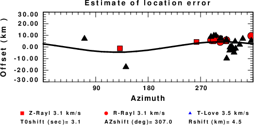
The derived shift in origin time and epicentral coordinates are given at the bottom of the figure.
Velocity Model
The WUS.model used for the waveform synthetic seismograms and for the surface wave eigenfunctions and dispersion is as follows
(The format is in the model96 format of Computer Programs in Seismology).
MODEL.01
Model after     8 iterations
ISOTROPIC
KGS
FLAT EARTH
1-D
CONSTANT VELOCITY
LINE08
LINE09
LINE10
LINE11
      H(KM)   VP(KM/S)   VS(KM/S) RHO(GM/CC)         QP         QS       ETAP       ETAS      FREFP      FREFS
     1.9000     3.4065     2.0089     2.2150  0.302E-02  0.679E-02   0.00       0.00       1.00       1.00
     6.1000     5.5445     3.2953     2.6089  0.349E-02  0.784E-02   0.00       0.00       1.00       1.00
    13.0000     6.2708     3.7396     2.7812  0.212E-02  0.476E-02   0.00       0.00       1.00       1.00
    19.0000     6.4075     3.7680     2.8223  0.111E-02  0.249E-02   0.00       0.00       1.00       1.00
     0.0000     7.9000     4.6200     3.2760  0.164E-10  0.370E-10   0.00       0.00       1.00       1.00
Last Changed Fri Apr 26 09:12:09 PM CDT 2024