Location
Location ANSS
The ANSS event ID is ak013bpso0xd and the event page is at
https://earthquake.usgs.gov/earthquakes/eventpage/ak013bpso0xd/executive.
2013/09/12 04:41:02 59.774 -152.831 11.3 4.1 Alaska
Focal Mechanism
 USGS/SLU Moment Tensor Solution
 ENS  2013/09/12 04:41:02:0  59.77 -152.83  11.3 4.1 Alaska

 Stations used:
   AK.BAL AK.BARN AK.BPAW AK.BRLK AK.BWN AK.CAST AK.CCB AK.CNP
   AK.CRQ AK.EYAK AK.FID AK.GHO AK.GLI AK.HIN AK.KIAG AK.KNK
   AK.KTH AK.MCK AK.MLY AK.NICH AK.PAX AK.PPLA AK.PTPK AK.RC01
   AK.SAW AK.SCM AK.SGA AK.SKN AK.SLK AK.SWD AK.TGL AK.WAX
   AT.SVW2 II.KDAK IM.IL31 TA.HDA TA.POKR TA.TCOL

 Filtering commands used:
   cut a -30 a 210
   rtr
   taper w 0.1
   hp c 0.02 n 3
   lp c 0.06 n 3

 Best Fitting Double Couple
  Mo = 1.60e+22 dyne-cm
  Mw = 4.07
  Z  = 19 km
  Plane   Strike  Dip  Rake
   NP1      205    81   -150
   NP2      110    60   -10
  Principal Axes:
   Axis    Value   Plunge  Azimuth
    T   1.60e+22     14     334
    N   0.00e+00     59     219
    P  -1.60e+22     27      72

 Moment Tensor: (dyne-cm)
    Component   Value
       Mxx     1.09e+22
       Mxy    -9.70e+21
       Mxz     1.39e+21
       Myy    -8.51e+21
       Myz    -7.89e+21
       Mzz    -2.41e+21


                     ##############
                 #   ###############---
              #### T #############--------
             #####   ############----------
           #####################-------------
          #####################---------------
         #####################-----------------
        -####################------------   ----
        --##################------------- P ----
       ----################--------------   -----
       ------#############-----------------------
       -------###########------------------------
       ----------#######-------------------------
        ------------####------------------------
        ---------------#------------------------
         -------------#######----------------##
          -----------#########################
           ----------########################
             -------#######################
              ------######################
                 --####################
                     ##############


 Global CMT Convention Moment Tensor:
      R          T          P
 -2.41e+21   1.39e+21   7.89e+21
  1.39e+21   1.09e+22   9.70e+21
  7.89e+21   9.70e+21  -8.51e+21


Details of the solution is found at

http://www.eas.slu.edu/eqc/eqc_mt/MECH.NA/20130912044102/index.html
|
Preferred Solution
The preferred solution from an analysis of the surface-wave spectral amplitude radiation pattern, waveform inversion or first motion observations is
      STK = 110
      DIP = 60
     RAKE = -10
       MW = 4.07
       HS = 19.0
The NDK file is 20130912044102.ndk
The waveform inversion is preferred.
Moment Tensor Comparison
The following compares this source inversion to those provided by others. The purpose is to look for major differences and also to note slight differences that might be inherent to the processing procedure. For completeness the USGS/SLU solution is repeated from above.
| SLU |
USGSMT |
 USGS/SLU Moment Tensor Solution
 ENS  2013/09/12 04:41:02:0  59.77 -152.83  11.3 4.1 Alaska

 Stations used:
   AK.BAL AK.BARN AK.BPAW AK.BRLK AK.BWN AK.CAST AK.CCB AK.CNP
   AK.CRQ AK.EYAK AK.FID AK.GHO AK.GLI AK.HIN AK.KIAG AK.KNK
   AK.KTH AK.MCK AK.MLY AK.NICH AK.PAX AK.PPLA AK.PTPK AK.RC01
   AK.SAW AK.SCM AK.SGA AK.SKN AK.SLK AK.SWD AK.TGL AK.WAX
   AT.SVW2 II.KDAK IM.IL31 TA.HDA TA.POKR TA.TCOL

 Filtering commands used:
   cut a -30 a 210
   rtr
   taper w 0.1
   hp c 0.02 n 3
   lp c 0.06 n 3

 Best Fitting Double Couple
  Mo = 1.60e+22 dyne-cm
  Mw = 4.07
  Z  = 19 km
  Plane   Strike  Dip  Rake
   NP1      205    81   -150
   NP2      110    60   -10
  Principal Axes:
   Axis    Value   Plunge  Azimuth
    T   1.60e+22     14     334
    N   0.00e+00     59     219
    P  -1.60e+22     27      72

 Moment Tensor: (dyne-cm)
    Component   Value
       Mxx     1.09e+22
       Mxy    -9.70e+21
       Mxz     1.39e+21
       Myy    -8.51e+21
       Myz    -7.89e+21
       Mzz    -2.41e+21


                     ##############
                 #   ###############---
              #### T #############--------
             #####   ############----------
           #####################-------------
          #####################---------------
         #####################-----------------
        -####################------------   ----
        --##################------------- P ----
       ----################--------------   -----
       ------#############-----------------------
       -------###########------------------------
       ----------#######-------------------------
        ------------####------------------------
        ---------------#------------------------
         -------------#######----------------##
          -----------#########################
           ----------########################
             -------#######################
              ------######################
                 --####################
                     ##############


 Global CMT Convention Moment Tensor:
      R          T          P
 -2.41e+21   1.39e+21   7.89e+21
  1.39e+21   1.09e+22   9.70e+21
  7.89e+21   9.70e+21  -8.51e+21


Details of the solution is found at

http://www.eas.slu.edu/eqc/eqc_mt/MECH.NA/20130912044102/index.html
|
Regional Moment Tensor (Mwr)

Moment magnitude derived from a moment tensor inversion of complete waveforms at regional distances (less than ~8 degrees), generally used for the analysis of small to moderate size earthquakes (typically Mw 3.5-6.0) crust or upper mantle earthquakes.

Moment
    2.05e+15 N-m
Magnitude
    4.1
Percent DC
    87%
Depth
    19.0 km
Updated
    2013-09-12 14:09:35 UTC
Author
    neic
Catalog
    ak
Contributor
    us
Code
    ak10804220-neic-mwr

Principal Axes
Axis	Value	Plunge	Azimuth
T	2.117	24	72
N	-0.135	65	242
P	-1.981	4	340
Nodal Planes
Plane	Strike	Dip	Rake
NP1	209	76	20
NP2	114	70	165
|

|
|
Magnitudes
Given the availability of digital waveforms for determination of the moment tensor, this section documents the added processing leading to mLg, if appropriate to the region, and ML by application of the respective IASPEI formulae. As a research study, the linear distance term of the IASPEI formula
for ML is adjusted to remove a linear distance trend in residuals to give a regionally defined ML. The defined ML uses horizontal component recordings, but the same procedure is applied to the vertical components since there may be some interest in vertical component ground motions. Residual plots versus distance may indicate interesting features of ground motion scaling in some distance ranges. A residual plot of the regionalized magnitude is given as a function of distance and azimuth, since data sets may transcend different wave propagation provinces.
ML Magnitude
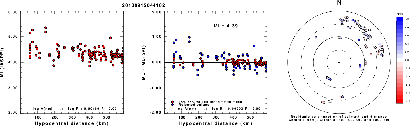
Left: ML computed using the IASPEI formula for Horizontal components. Center: ML residuals computed using a modified IASPEI formula that accounts for path specific attenuation; the values used for the trimmed mean are indicated. The ML relation used for each figure is given at the bottom of each plot.
Right: Residuals from new relation as a function of distance and azimuth.
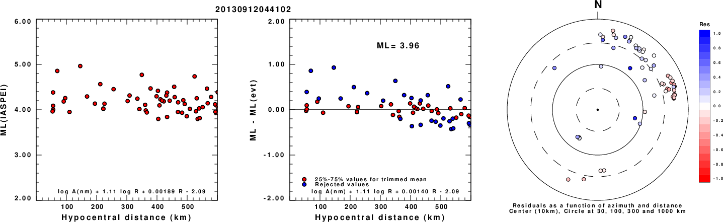
Left: ML computed using the IASPEI formula for Vertical components (research). Center: ML residuals computed using a modified IASPEI formula that accounts for path specific attenuation; the values used for the trimmed mean are indicated. The ML relation used for each figure is given at the bottom of each plot.
Right: Residuals from new relation as a function of distance and azimuth.
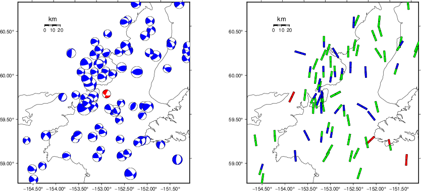
Context
The left panel of the next figure presents the focal mechanism for this earthquake (red) in the context of other nearby events (blue) in the SLU Moment Tensor Catalog. The right panel shows the inferred direction of maximum compressive stress and the type of faulting (green is strike-slip, red is normal, blue is thrust; oblique is shown by a combination of colors). Thus context plot is useful for assessing the appropriateness of the moment tensor of this event.
Waveform Inversion using wvfgrd96
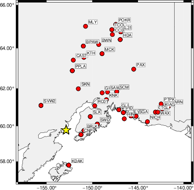
The focal mechanism was determined using broadband seismic waveforms. The location of the event (star) and the
stations used for (red) the waveform inversion are shown in the next figure.
|
|
Location of broadband stations used for waveform inversion
|
The program wvfgrd96 was used with good traces observed at short distance to determine the focal mechanism, depth and seismic moment. This technique requires a high quality signal and well determined velocity model for the Green's functions. To the extent that these are the quality data, this type of mechanism should be preferred over the radiation pattern technique which requires the separate step of defining the pressure and tension quadrants and the correct strike.
The observed and predicted traces are filtered using the following gsac commands:
cut a -30 a 210
rtr
taper w 0.1
hp c 0.02 n 3
lp c 0.06 n 3
The results of this grid search are as follow:
           DEPTH  STK   DIP  RAKE   MW    FIT
WVFGRD96    1.0   225    45   -80   3.72 0.3115
WVFGRD96    2.0    55    45   -95   3.86 0.3956
WVFGRD96    3.0    25    70   -35   3.84 0.3896
WVFGRD96    4.0    30    80   -30   3.87 0.4038
WVFGRD96    5.0    30    85   -30   3.90 0.4223
WVFGRD96    6.0    30    85   -30   3.92 0.4426
WVFGRD96    7.0   210    90    25   3.93 0.4634
WVFGRD96    8.0    30    90   -35   3.98 0.4837
WVFGRD96    9.0    30    90   -30   3.99 0.4969
WVFGRD96   10.0   105    50   -15   3.97 0.5158
WVFGRD96   11.0   105    50   -15   3.98 0.5297
WVFGRD96   12.0   110    55   -15   4.01 0.5419
WVFGRD96   13.0   110    55   -10   4.01 0.5513
WVFGRD96   14.0   110    55   -10   4.02 0.5582
WVFGRD96   15.0   110    55   -10   4.03 0.5631
WVFGRD96   16.0   110    60   -15   4.05 0.5678
WVFGRD96   17.0   110    60   -15   4.06 0.5711
WVFGRD96   18.0   110    60   -15   4.07 0.5725
WVFGRD96   19.0   110    60   -10   4.07 0.5730
WVFGRD96   20.0   115    60    10   4.08 0.5724
WVFGRD96   21.0   115    60    10   4.09 0.5700
WVFGRD96   22.0   115    60    10   4.10 0.5682
WVFGRD96   23.0   115    60    10   4.10 0.5648
WVFGRD96   24.0   115    60    10   4.11 0.5593
WVFGRD96   25.0   115    60    15   4.11 0.5542
WVFGRD96   26.0   115    60    15   4.12 0.5471
WVFGRD96   27.0   115    60    15   4.12 0.5390
WVFGRD96   28.0   115    60    15   4.13 0.5311
WVFGRD96   29.0   115    60    15   4.13 0.5197
WVFGRD96   30.0   115    60    20   4.13 0.5106
WVFGRD96   31.0   115    65    20   4.15 0.5011
WVFGRD96   32.0   115    65    20   4.15 0.4891
WVFGRD96   33.0   115    65    20   4.16 0.4797
WVFGRD96   34.0   115    65    25   4.16 0.4699
WVFGRD96   35.0   115    65    25   4.16 0.4617
WVFGRD96   36.0   115    65    25   4.17 0.4544
WVFGRD96   37.0   115    65    25   4.18 0.4468
WVFGRD96   38.0   115    65    25   4.19 0.4408
WVFGRD96   39.0   115    65    25   4.20 0.4358
WVFGRD96   40.0   110    60   -25   4.30 0.4396
WVFGRD96   41.0   110    60   -25   4.30 0.4390
WVFGRD96   42.0   110    60   -25   4.31 0.4384
WVFGRD96   43.0   110    60   -25   4.32 0.4379
WVFGRD96   44.0   110    60   -25   4.33 0.4371
WVFGRD96   45.0   110    60   -20   4.33 0.4365
WVFGRD96   46.0   110    65   -25   4.34 0.4358
WVFGRD96   47.0   110    65   -25   4.35 0.4351
WVFGRD96   48.0   110    65   -25   4.35 0.4341
WVFGRD96   49.0   110    65   -20   4.35 0.4326
The best solution is
WVFGRD96 19.0 110 60 -10 4.07 0.5730
The mechanism corresponding to the best fit is
|
|
Figure 1. Waveform inversion focal mechanism
|
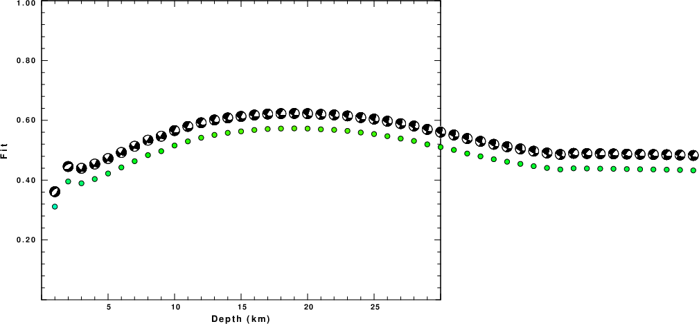
The best fit as a function of depth is given in the following figure:
|
|
Figure 2. Depth sensitivity for waveform mechanism
|
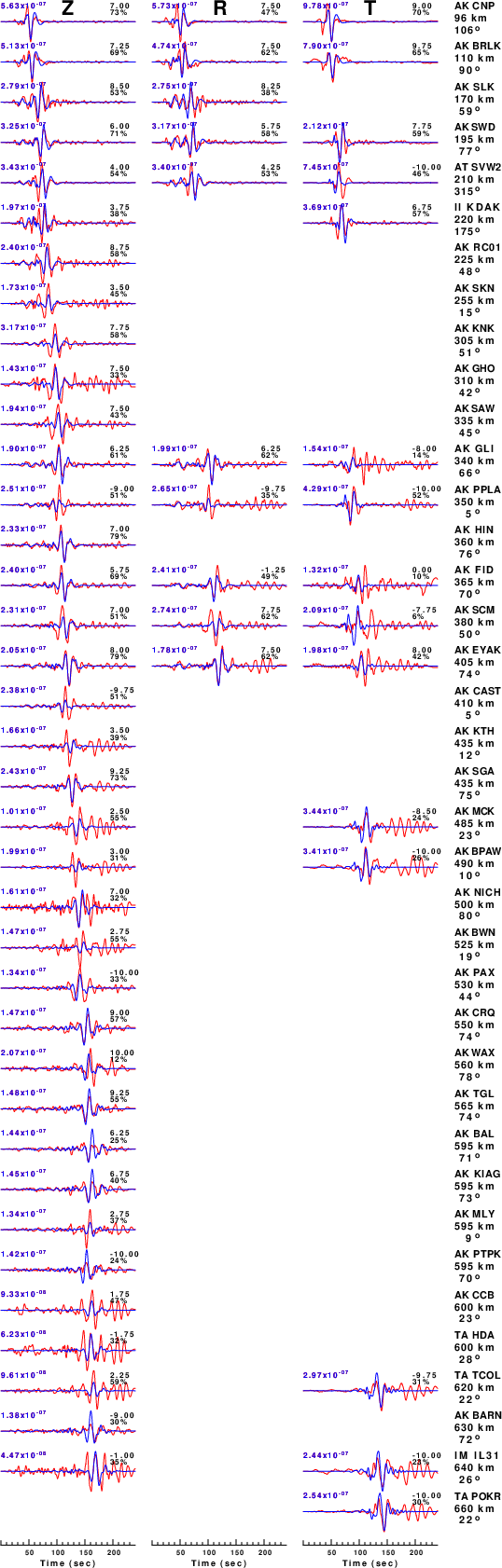
The comparison of the observed and predicted waveforms is given in the next figure. The red traces are the observed and the blue are the predicted.
Each observed-predicted component is plotted to the same scale and peak amplitudes are indicated by the numbers to the left of each trace. A pair of numbers is given in black at the right of each predicted traces. The upper number it the time shift required for maximum correlation between the observed and predicted traces. This time shift is required because the synthetics are not computed at exactly the same distance as the observed, the velocity model used in the predictions may not be perfect and the epicentral parameters may be be off.
A positive time shift indicates that the prediction is too fast and should be delayed to match the observed trace (shift to the right in this figure). A negative value indicates that the prediction is too slow. The lower number gives the percentage of variance reduction to characterize the individual goodness of fit (100% indicates a perfect fit).
The bandpass filter used in the processing and for the display was
cut a -30 a 210
rtr
taper w 0.1
hp c 0.02 n 3
lp c 0.06 n 3
|
|
Figure 3. Waveform comparison for selected depth. Red: observed; Blue - predicted. The time shift with respect to the model prediction is indicated. The percent of fit is also indicated. The time scale is relative to the first trace sample.
|
|
|
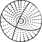
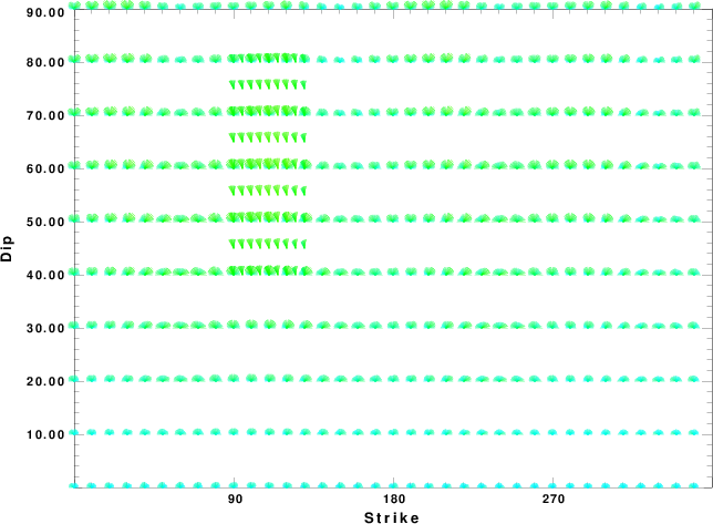
Focal mechanism sensitivity at the preferred depth. The red color indicates a very good fit to the waveforms.
Each solution is plotted as a vector at a given value of strike and dip with the angle of the vector representing the rake angle, measured, with respect to the upward vertical (N) in the figure.
|
A check on the assumed source location is possible by looking at the time shifts between the observed and predicted traces. The time shifts for waveform matching arise for several reasons:
- The origin time and epicentral distance are incorrect
- The velocity model used for the inversion is incorrect
- The velocity model used to define the P-arrival time is not the
same as the velocity model used for the waveform inversion
(assuming that the initial trace alignment is based on the
P arrival time)
Assuming only a mislocation, the time shifts are fit to a functional form:
Time_shift = A + B cos Azimuth + C Sin Azimuth
The time shifts for this inversion lead to the next figure:
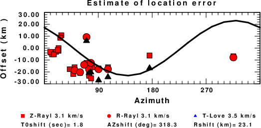
The derived shift in origin time and epicentral coordinates are given at the bottom of the figure.
Velocity Model
The WUS.model used for the waveform synthetic seismograms and for the surface wave eigenfunctions and dispersion is as follows
(The format is in the model96 format of Computer Programs in Seismology).
MODEL.01
Model after     8 iterations
ISOTROPIC
KGS
FLAT EARTH
1-D
CONSTANT VELOCITY
LINE08
LINE09
LINE10
LINE11
      H(KM)   VP(KM/S)   VS(KM/S) RHO(GM/CC)         QP         QS       ETAP       ETAS      FREFP      FREFS
     1.9000     3.4065     2.0089     2.2150  0.302E-02  0.679E-02   0.00       0.00       1.00       1.00
     6.1000     5.5445     3.2953     2.6089  0.349E-02  0.784E-02   0.00       0.00       1.00       1.00
    13.0000     6.2708     3.7396     2.7812  0.212E-02  0.476E-02   0.00       0.00       1.00       1.00
    19.0000     6.4075     3.7680     2.8223  0.111E-02  0.249E-02   0.00       0.00       1.00       1.00
     0.0000     7.9000     4.6200     3.2760  0.164E-10  0.370E-10   0.00       0.00       1.00       1.00
Last Changed Fri Apr 26 08:33:01 PM CDT 2024