Location
Location ANSS
The ANSS event ID is ak013bo3451v and the event page is at
https://earthquake.usgs.gov/earthquakes/eventpage/ak013bo3451v/executive.
2013/09/11 01:02:59 61.348 -149.512 41.3 4 Alaska
Focal Mechanism
 USGS/SLU Moment Tensor Solution
 ENS  2013/09/11 01:02:59:0  61.35 -149.51  41.3 4.0 Alaska

 Stations used:
   AK.CAPN AK.CAST AK.EYAK AK.GLI AK.HDA AK.KNK AK.PAX AK.PPLA
   AK.PTPK AK.RC01 AK.SAW AK.SCM AK.SKN AK.SLK AK.SWD AK.TGL
   AK.WAT1 AK.WAT2 AK.WAT3 AK.WAT4 AK.WAT6 AK.WAT7 AK.WAX

 Filtering commands used:
   cut a -30 a 180
   rtr
   taper w 0.1
   hp c 0.02 n 3
   lp c 0.06 n 3

 Best Fitting Double Couple
  Mo = 1.22e+22 dyne-cm
  Mw = 3.99
  Z  = 45 km
  Plane   Strike  Dip  Rake
   NP1      143    57   -130
   NP2       20    50   -45
  Principal Axes:
   Axis    Value   Plunge  Azimuth
    T   1.22e+22      4     260
    N   0.00e+00     33     167
    P  -1.22e+22     57     356

 Moment Tensor: (dyne-cm)
    Component   Value
       Mxx    -3.24e+21
       Mxy     2.32e+21
       Mxz    -5.71e+21
       Myy     1.17e+22
       Myz    -4.87e+20
       Mzz    -8.47e+21


                     --------------
                 -------------------###
              #----------------------#####
             ##-----------------------#####
           ####------------------------######
          #####-----------   ----------#######
         ######----------- P ----------########
        ########----------   ----------#########
        ########-----------------------#########
       ##########----------------------##########
       ###########---------------------##########
       ############-------------------###########
          ##########------------------###########
        T ###########----------------###########
          #############-------------############
         ###############-----------############
          ################--------############
           #################-----############
             ##############################
              ###############-------######
                 #########-------------
                     --------------


 Global CMT Convention Moment Tensor:
      R          T          P
 -8.47e+21  -5.71e+21   4.87e+20
 -5.71e+21  -3.24e+21  -2.32e+21
  4.87e+20  -2.32e+21   1.17e+22


Details of the solution is found at

http://www.eas.slu.edu/eqc/eqc_mt/MECH.NA/20130911010259/index.html
|
Preferred Solution
The preferred solution from an analysis of the surface-wave spectral amplitude radiation pattern, waveform inversion or first motion observations is
      STK = 20
      DIP = 50
     RAKE = -45
       MW = 3.99
       HS = 45.0
The NDK file is 20130911010259.ndk
The waveform inversion is preferred.
Magnitudes
Given the availability of digital waveforms for determination of the moment tensor, this section documents the added processing leading to mLg, if appropriate to the region, and ML by application of the respective IASPEI formulae. As a research study, the linear distance term of the IASPEI formula
for ML is adjusted to remove a linear distance trend in residuals to give a regionally defined ML. The defined ML uses horizontal component recordings, but the same procedure is applied to the vertical components since there may be some interest in vertical component ground motions. Residual plots versus distance may indicate interesting features of ground motion scaling in some distance ranges. A residual plot of the regionalized magnitude is given as a function of distance and azimuth, since data sets may transcend different wave propagation provinces.
ML Magnitude
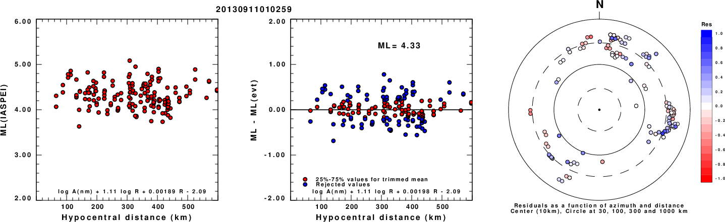
Left: ML computed using the IASPEI formula for Horizontal components. Center: ML residuals computed using a modified IASPEI formula that accounts for path specific attenuation; the values used for the trimmed mean are indicated. The ML relation used for each figure is given at the bottom of each plot.
Right: Residuals from new relation as a function of distance and azimuth.
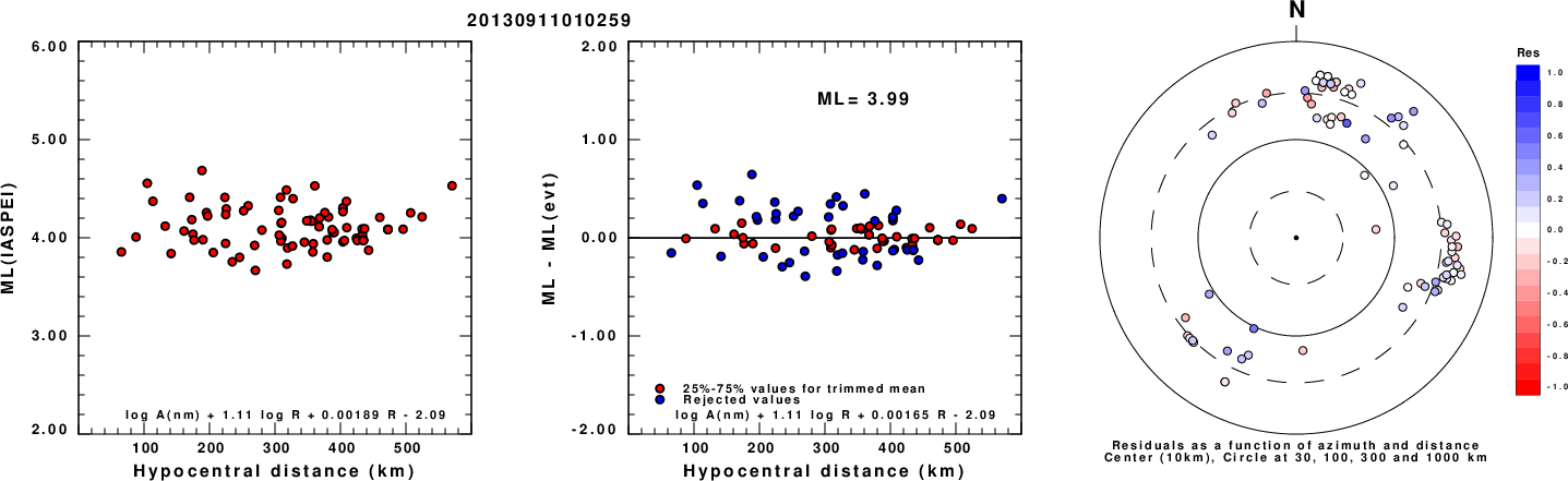
Left: ML computed using the IASPEI formula for Vertical components (research). Center: ML residuals computed using a modified IASPEI formula that accounts for path specific attenuation; the values used for the trimmed mean are indicated. The ML relation used for each figure is given at the bottom of each plot.
Right: Residuals from new relation as a function of distance and azimuth.
Context
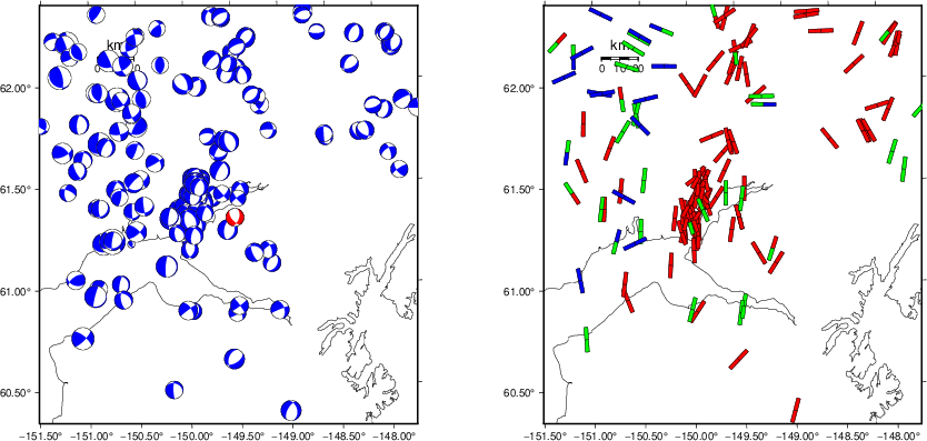
The left panel of the next figure presents the focal mechanism for this earthquake (red) in the context of other nearby events (blue) in the SLU Moment Tensor Catalog. The right panel shows the inferred direction of maximum compressive stress and the type of faulting (green is strike-slip, red is normal, blue is thrust; oblique is shown by a combination of colors). Thus context plot is useful for assessing the appropriateness of the moment tensor of this event.
Waveform Inversion using wvfgrd96
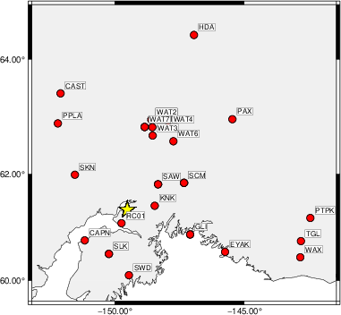
The focal mechanism was determined using broadband seismic waveforms. The location of the event (star) and the
stations used for (red) the waveform inversion are shown in the next figure.
|
|
Location of broadband stations used for waveform inversion
|
The program wvfgrd96 was used with good traces observed at short distance to determine the focal mechanism, depth and seismic moment. This technique requires a high quality signal and well determined velocity model for the Green's functions. To the extent that these are the quality data, this type of mechanism should be preferred over the radiation pattern technique which requires the separate step of defining the pressure and tension quadrants and the correct strike.
The observed and predicted traces are filtered using the following gsac commands:
cut a -30 a 180
rtr
taper w 0.1
hp c 0.02 n 3
lp c 0.06 n 3
The results of this grid search are as follow:
           DEPTH  STK   DIP  RAKE   MW    FIT
WVFGRD96    0.5   170    45    95   3.25 0.1964
WVFGRD96    1.0   345    45    90   3.29 0.1977
WVFGRD96    2.0   170    45    95   3.40 0.2549
WVFGRD96    3.0   345    45    90   3.47 0.2651
WVFGRD96    4.0   135    80   -20   3.47 0.2450
WVFGRD96    5.0   130    70   -30   3.51 0.2545
WVFGRD96    6.0   130    70   -30   3.52 0.2616
WVFGRD96    7.0   130    70   -25   3.54 0.2693
WVFGRD96    8.0   130    70   -30   3.58 0.2738
WVFGRD96    9.0   130    70   -30   3.59 0.2747
WVFGRD96   10.0   130    85   -40   3.56 0.2793
WVFGRD96   11.0   130    85   -40   3.57 0.2898
WVFGRD96   12.0    45    45    25   3.57 0.3051
WVFGRD96   13.0    45    50    25   3.60 0.3256
WVFGRD96   14.0    45    50    25   3.61 0.3444
WVFGRD96   15.0    45    50    25   3.62 0.3614
WVFGRD96   16.0    45    55    20   3.64 0.3775
WVFGRD96   17.0    45    55    20   3.66 0.3927
WVFGRD96   18.0    45    55    20   3.67 0.4065
WVFGRD96   19.0    40    55    15   3.67 0.4191
WVFGRD96   20.0    40    55    15   3.68 0.4308
WVFGRD96   21.0    40    55    15   3.70 0.4417
WVFGRD96   22.0    30    55   -20   3.71 0.4551
WVFGRD96   23.0    30    55   -20   3.72 0.4677
WVFGRD96   24.0    30    60   -25   3.74 0.4804
WVFGRD96   25.0    30    60   -25   3.75 0.4923
WVFGRD96   26.0    30    60   -25   3.76 0.5038
WVFGRD96   27.0    30    60   -25   3.77 0.5147
WVFGRD96   28.0    25    60   -30   3.78 0.5256
WVFGRD96   29.0    25    60   -30   3.78 0.5366
WVFGRD96   30.0    25    60   -30   3.79 0.5470
WVFGRD96   31.0    25    60   -30   3.80 0.5567
WVFGRD96   32.0    25    60   -30   3.81 0.5657
WVFGRD96   33.0    25    60   -30   3.82 0.5740
WVFGRD96   34.0    25    60   -30   3.83 0.5810
WVFGRD96   35.0    25    60   -30   3.84 0.5865
WVFGRD96   36.0    25    60   -30   3.85 0.5909
WVFGRD96   37.0    25    60   -30   3.86 0.5934
WVFGRD96   38.0    25    60   -30   3.87 0.5941
WVFGRD96   39.0    25    60   -30   3.88 0.5924
WVFGRD96   40.0    20    50   -40   3.95 0.6031
WVFGRD96   41.0    20    50   -40   3.96 0.6085
WVFGRD96   42.0    20    50   -45   3.98 0.6119
WVFGRD96   43.0    20    50   -45   3.98 0.6143
WVFGRD96   44.0    20    50   -45   3.99 0.6155
WVFGRD96   45.0    20    50   -45   3.99 0.6162
WVFGRD96   46.0    20    50   -45   4.00 0.6157
WVFGRD96   47.0    20    50   -45   4.01 0.6148
WVFGRD96   48.0    20    50   -40   4.01 0.6134
WVFGRD96   49.0    20    50   -40   4.01 0.6120
WVFGRD96   50.0    20    50   -40   4.02 0.6100
WVFGRD96   51.0    20    50   -40   4.02 0.6079
WVFGRD96   52.0    20    50   -40   4.03 0.6059
WVFGRD96   53.0    20    50   -40   4.03 0.6031
WVFGRD96   54.0    20    50   -40   4.03 0.6007
WVFGRD96   55.0    20    50   -40   4.04 0.5978
WVFGRD96   56.0    25    50   -35   4.04 0.5954
WVFGRD96   57.0    25    50   -35   4.05 0.5934
WVFGRD96   58.0    25    50   -35   4.05 0.5915
WVFGRD96   59.0    25    50   -35   4.06 0.5892
WVFGRD96   60.0    25    50   -35   4.06 0.5871
WVFGRD96   61.0    25    50   -35   4.06 0.5848
WVFGRD96   62.0    25    50   -35   4.07 0.5820
WVFGRD96   63.0    25    50   -35   4.07 0.5791
WVFGRD96   64.0    25    50   -35   4.08 0.5762
WVFGRD96   65.0    30    50   -30   4.08 0.5737
WVFGRD96   66.0    30    50   -30   4.09 0.5714
WVFGRD96   67.0    30    50   -30   4.09 0.5692
WVFGRD96   68.0    30    50   -30   4.09 0.5671
WVFGRD96   69.0    30    50   -30   4.10 0.5641
WVFGRD96   70.0    30    50   -30   4.10 0.5613
WVFGRD96   71.0    30    50   -25   4.10 0.5585
WVFGRD96   72.0    30    50   -25   4.10 0.5555
WVFGRD96   73.0    30    50   -25   4.11 0.5529
WVFGRD96   74.0    30    50   -25   4.11 0.5496
WVFGRD96   75.0    30    50   -25   4.11 0.5460
WVFGRD96   76.0    30    45   -25   4.11 0.5435
WVFGRD96   77.0    30    45   -25   4.11 0.5407
WVFGRD96   78.0    30    45   -25   4.12 0.5382
WVFGRD96   79.0    30    45   -25   4.12 0.5354
WVFGRD96   80.0    30    45   -25   4.12 0.5324
WVFGRD96   81.0    30    45   -25   4.13 0.5294
WVFGRD96   82.0    30    45   -25   4.13 0.5258
WVFGRD96   83.0    30    45   -25   4.13 0.5230
WVFGRD96   84.0    30    45   -25   4.14 0.5193
WVFGRD96   85.0    30    45   -25   4.14 0.5159
WVFGRD96   86.0    30    45   -25   4.14 0.5123
WVFGRD96   87.0    30    45   -25   4.14 0.5086
WVFGRD96   88.0    30    45   -25   4.14 0.5046
WVFGRD96   89.0    30    45   -25   4.15 0.5012
WVFGRD96   90.0    35    45   -20   4.16 0.4975
WVFGRD96   91.0    35    45   -20   4.16 0.4937
WVFGRD96   92.0    35    45   -20   4.16 0.4901
WVFGRD96   93.0    35    45   -20   4.17 0.4864
WVFGRD96   94.0    35    45   -20   4.17 0.4824
WVFGRD96   95.0    35    45   -20   4.17 0.4788
WVFGRD96   96.0    35    45   -20   4.17 0.4744
WVFGRD96   97.0    35    45   -20   4.17 0.4707
WVFGRD96   98.0    35    45   -20   4.17 0.4664
WVFGRD96   99.0    35    45   -20   4.18 0.4625
The best solution is
WVFGRD96 45.0 20 50 -45 3.99 0.6162
The mechanism corresponding to the best fit is
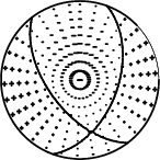
|
|
Figure 1. Waveform inversion focal mechanism
|
The best fit as a function of depth is given in the following figure:
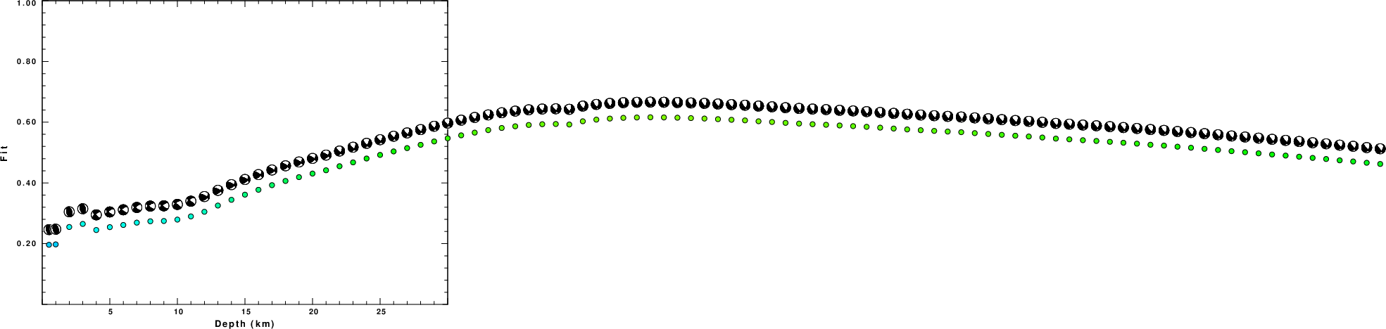
|
|
Figure 2. Depth sensitivity for waveform mechanism
|
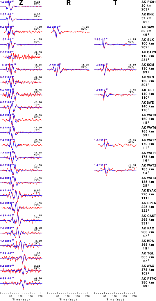
The comparison of the observed and predicted waveforms is given in the next figure. The red traces are the observed and the blue are the predicted.
Each observed-predicted component is plotted to the same scale and peak amplitudes are indicated by the numbers to the left of each trace. A pair of numbers is given in black at the right of each predicted traces. The upper number it the time shift required for maximum correlation between the observed and predicted traces. This time shift is required because the synthetics are not computed at exactly the same distance as the observed, the velocity model used in the predictions may not be perfect and the epicentral parameters may be be off.
A positive time shift indicates that the prediction is too fast and should be delayed to match the observed trace (shift to the right in this figure). A negative value indicates that the prediction is too slow. The lower number gives the percentage of variance reduction to characterize the individual goodness of fit (100% indicates a perfect fit).
The bandpass filter used in the processing and for the display was
cut a -30 a 180
rtr
taper w 0.1
hp c 0.02 n 3
lp c 0.06 n 3
|
|
Figure 3. Waveform comparison for selected depth. Red: observed; Blue - predicted. The time shift with respect to the model prediction is indicated. The percent of fit is also indicated. The time scale is relative to the first trace sample.
|
|
|
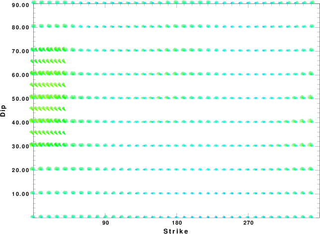
Focal mechanism sensitivity at the preferred depth. The red color indicates a very good fit to the waveforms.
Each solution is plotted as a vector at a given value of strike and dip with the angle of the vector representing the rake angle, measured, with respect to the upward vertical (N) in the figure.
|
A check on the assumed source location is possible by looking at the time shifts between the observed and predicted traces. The time shifts for waveform matching arise for several reasons:
- The origin time and epicentral distance are incorrect
- The velocity model used for the inversion is incorrect
- The velocity model used to define the P-arrival time is not the
same as the velocity model used for the waveform inversion
(assuming that the initial trace alignment is based on the
P arrival time)
Assuming only a mislocation, the time shifts are fit to a functional form:
Time_shift = A + B cos Azimuth + C Sin Azimuth
The time shifts for this inversion lead to the next figure:
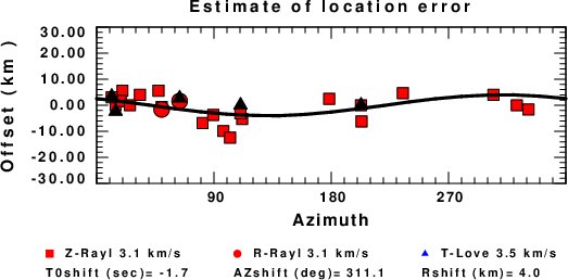
The derived shift in origin time and epicentral coordinates are given at the bottom of the figure.
Velocity Model
The WUS.model used for the waveform synthetic seismograms and for the surface wave eigenfunctions and dispersion is as follows
(The format is in the model96 format of Computer Programs in Seismology).
MODEL.01
Model after     8 iterations
ISOTROPIC
KGS
FLAT EARTH
1-D
CONSTANT VELOCITY
LINE08
LINE09
LINE10
LINE11
      H(KM)   VP(KM/S)   VS(KM/S) RHO(GM/CC)         QP         QS       ETAP       ETAS      FREFP      FREFS
     1.9000     3.4065     2.0089     2.2150  0.302E-02  0.679E-02   0.00       0.00       1.00       1.00
     6.1000     5.5445     3.2953     2.6089  0.349E-02  0.784E-02   0.00       0.00       1.00       1.00
    13.0000     6.2708     3.7396     2.7812  0.212E-02  0.476E-02   0.00       0.00       1.00       1.00
    19.0000     6.4075     3.7680     2.8223  0.111E-02  0.249E-02   0.00       0.00       1.00       1.00
     0.0000     7.9000     4.6200     3.2760  0.164E-10  0.370E-10   0.00       0.00       1.00       1.00
Last Changed Fri Apr 26 08:22:53 PM CDT 2024