Location
Location ANSS
The ANSS event ID is ak013azm6wlj and the event page is at
https://earthquake.usgs.gov/earthquakes/eventpage/ak013azm6wlj/executive.
2013/08/27 21:41:33 63.205 -150.604 129.5 5 Alaska
Focal Mechanism
 USGS/SLU Moment Tensor Solution
 ENS  2013/08/27 21:41:33:0  63.21 -150.60 129.5 5.0 Alaska

 Stations used:
   AK.COLD AK.DOT AK.PAX AK.PPLA AK.SWD AT.MENT AT.PMR AT.SVW2
   AT.TTA

 Filtering commands used:
   cut a -30 a 120
   rtr
   taper w 0.1
   hp c 0.02 n 3
   lp c 0.05 n 3

 Best Fitting Double Couple
  Mo = 2.37e+23 dyne-cm
  Mw = 4.85
  Z  = 137 km
  Plane   Strike  Dip  Rake
   NP1       16    87   110
   NP2      115    20    10
  Principal Axes:
   Axis    Value   Plunge  Azimuth
    T   2.37e+23     45     305
    N   0.00e+00     20     194
    P  -2.37e+23     38      88

 Moment Tensor: (dyne-cm)
    Component   Value
       Mxx     3.94e+22
       Mxy    -6.15e+22
       Mxz     6.42e+22
       Myy    -6.59e+22
       Myz    -2.12e+23
       Mzz     2.65e+22


                     ############--
                 ################------
              ###################---------
             ###################-----------
           #####################-------------
          ######################--------------
         ########   ###########----------------
        -######## T ###########-----------------
        -########   ##########------------------
       --#####################---------   -------
       --####################---------- P -------
       --####################----------   -------
       ---##################---------------------
        --##################--------------------
        ---################---------------------
         ---##############---------------------
          ----############--------------------
           -----#########-------------------#
             -----#######-----------------#
              --------##--------------####
                 ------################
                     --############


 Global CMT Convention Moment Tensor:
      R          T          P
  2.65e+22   6.42e+22   2.12e+23
  6.42e+22   3.94e+22   6.15e+22
  2.12e+23   6.15e+22  -6.59e+22


Details of the solution is found at

http://www.eas.slu.edu/eqc/eqc_mt/MECH.NA/20130827214133/index.html
|
Preferred Solution
The preferred solution from an analysis of the surface-wave spectral amplitude radiation pattern, waveform inversion or first motion observations is
      STK = 115
      DIP = 20
     RAKE = 10
       MW = 4.85
       HS = 137.0
The NDK file is 20130827214133.ndk
The waveform inversion is preferred.
Moment Tensor Comparison
The following compares this source inversion to those provided by others. The purpose is to look for major differences and also to note slight differences that might be inherent to the processing procedure. For completeness the USGS/SLU solution is repeated from above.
| SLU |
USGSMT |
 USGS/SLU Moment Tensor Solution
 ENS  2013/08/27 21:41:33:0  63.21 -150.60 129.5 5.0 Alaska

 Stations used:
   AK.COLD AK.DOT AK.PAX AK.PPLA AK.SWD AT.MENT AT.PMR AT.SVW2
   AT.TTA

 Filtering commands used:
   cut a -30 a 120
   rtr
   taper w 0.1
   hp c 0.02 n 3
   lp c 0.05 n 3

 Best Fitting Double Couple
  Mo = 2.37e+23 dyne-cm
  Mw = 4.85
  Z  = 137 km
  Plane   Strike  Dip  Rake
   NP1       16    87   110
   NP2      115    20    10
  Principal Axes:
   Axis    Value   Plunge  Azimuth
    T   2.37e+23     45     305
    N   0.00e+00     20     194
    P  -2.37e+23     38      88

 Moment Tensor: (dyne-cm)
    Component   Value
       Mxx     3.94e+22
       Mxy    -6.15e+22
       Mxz     6.42e+22
       Myy    -6.59e+22
       Myz    -2.12e+23
       Mzz     2.65e+22


                     ############--
                 ################------
              ###################---------
             ###################-----------
           #####################-------------
          ######################--------------
         ########   ###########----------------
        -######## T ###########-----------------
        -########   ##########------------------
       --#####################---------   -------
       --####################---------- P -------
       --####################----------   -------
       ---##################---------------------
        --##################--------------------
        ---################---------------------
         ---##############---------------------
          ----############--------------------
           -----#########-------------------#
             -----#######-----------------#
              --------##--------------####
                 ------################
                     --############


 Global CMT Convention Moment Tensor:
      R          T          P
  2.65e+22   6.42e+22   2.12e+23
  6.42e+22   3.94e+22   6.15e+22
  2.12e+23   6.15e+22  -6.59e+22


Details of the solution is found at

http://www.eas.slu.edu/eqc/eqc_mt/MECH.NA/20130827214133/index.html
|
us usb000jce7_Mww

Type Mww
Moment 2.48e+16 N-m
Magnitude 4.9
Percent DC 86%
Depth 130.0 km
Author us
Updated 2013-08-27 23:05:45 UTC

Principal Axes

Axis	Value	Plunge	Azimuth
T	2.397	37°	269°
N	0.159	16°	11°
P	-2.556	48°	120°
Nodal Planes

Plane	Strike	Dip	Rake
NP1	193°	84°	-74°
NP2	302°	17°	-160°
 in the context of other nearby events (blue) in the SLU Moment Tensor Catalog. The right panel shows the inferred direction of maximum compressive stress and the type of faulting (green is strike-slip, red is normal, blue is thrust; oblique is shown by a combination of colors). Thus context plot is useful for assessing the appropriateness of the moment tensor of this event.
<br>
<table>
<tr><td><img src=) |
Waveform Inversion using wvfgrd96
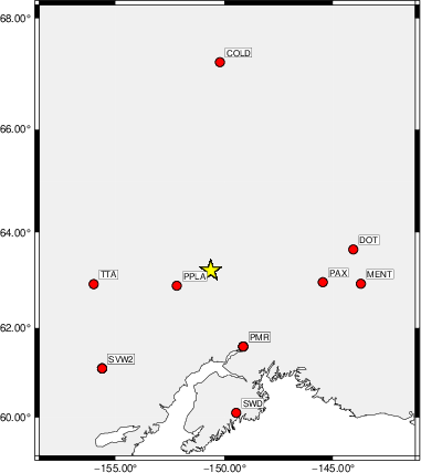
The focal mechanism was determined using broadband seismic waveforms. The location of the event (star) and the
stations used for (red) the waveform inversion are shown in the next figure.
|
|
Location of broadband stations used for waveform inversion
|
The program wvfgrd96 was used with good traces observed at short distance to determine the focal mechanism, depth and seismic moment. This technique requires a high quality signal and well determined velocity model for the Green's functions. To the extent that these are the quality data, this type of mechanism should be preferred over the radiation pattern technique which requires the separate step of defining the pressure and tension quadrants and the correct strike.
The observed and predicted traces are filtered using the following gsac commands:
cut a -30 a 120
rtr
taper w 0.1
hp c 0.02 n 3
lp c 0.05 n 3
The results of this grid search are as follow:
           DEPTH  STK   DIP  RAKE   MW    FIT
WVFGRD96    0.5   320    50   -70   3.84 0.1840
WVFGRD96    1.0   130    40   -85   3.88 0.1996
WVFGRD96    2.0   130    40   -85   3.97 0.2398
WVFGRD96    3.0   140    40   -75   4.04 0.2653
WVFGRD96    4.0   145    40   -70   4.08 0.2591
WVFGRD96    5.0    10    80    15   4.11 0.2632
WVFGRD96    6.0    10    80    10   4.15 0.2783
WVFGRD96    7.0    10    80    10   4.18 0.2958
WVFGRD96    8.0    10    80    10   4.22 0.3067
WVFGRD96    9.0    15    75    10   4.25 0.3191
WVFGRD96   10.0    15    75    10   4.28 0.3275
WVFGRD96   11.0    10    80    10   4.29 0.3296
WVFGRD96   12.0    10    80    10   4.30 0.3283
WVFGRD96   13.0    10    80    10   4.31 0.3249
WVFGRD96   14.0    10    80    10   4.32 0.3226
WVFGRD96   15.0    10    80    10   4.32 0.3243
WVFGRD96   16.0    10    80    15   4.31 0.3250
WVFGRD96   17.0    10    80    15   4.31 0.3255
WVFGRD96   18.0    10    80    15   4.32 0.3256
WVFGRD96   19.0    10    80    15   4.32 0.3257
WVFGRD96   20.0    10    80    15   4.33 0.3269
WVFGRD96   21.0    10    85    15   4.35 0.3264
WVFGRD96   22.0    10    85    15   4.35 0.3276
WVFGRD96   23.0    10    85    15   4.35 0.3295
WVFGRD96   24.0    10    85    15   4.36 0.3282
WVFGRD96   25.0    10    85    15   4.36 0.3292
WVFGRD96   26.0    10    85    20   4.34 0.3292
WVFGRD96   27.0    10    85    20   4.35 0.3312
WVFGRD96   28.0   185    90   -20   4.36 0.3314
WVFGRD96   29.0   185    90   -20   4.36 0.3320
WVFGRD96   30.0     5    90    20   4.37 0.3343
WVFGRD96   31.0     5    90    20   4.37 0.3352
WVFGRD96   32.0     5    90    20   4.38 0.3343
WVFGRD96   33.0   185    90   -20   4.39 0.3344
WVFGRD96   34.0     5    90    20   4.39 0.3353
WVFGRD96   35.0   190    90   -20   4.40 0.3341
WVFGRD96   36.0    10    90    15   4.44 0.3335
WVFGRD96   37.0   190    90   -15   4.45 0.3321
WVFGRD96   38.0   190    90   -15   4.46 0.3329
WVFGRD96   39.0    10    85    10   4.49 0.3345
WVFGRD96   40.0   280    85   -10   4.55 0.3407
WVFGRD96   41.0   280    85   -10   4.56 0.3478
WVFGRD96   42.0   280    85   -10   4.57 0.3547
WVFGRD96   43.0   280    85   -10   4.58 0.3615
WVFGRD96   44.0   280    85   -10   4.58 0.3679
WVFGRD96   45.0   100    90    10   4.60 0.3690
WVFGRD96   46.0   100    90    10   4.61 0.3768
WVFGRD96   47.0   100    90    10   4.62 0.3843
WVFGRD96   48.0   100    90    10   4.62 0.3912
WVFGRD96   49.0   280    85    -5   4.63 0.4022
WVFGRD96   50.0   100    90    10   4.63 0.4036
WVFGRD96   51.0   280    85    -5   4.64 0.4162
WVFGRD96   52.0   100    90     5   4.66 0.4191
WVFGRD96   53.0   100    90     5   4.66 0.4256
WVFGRD96   54.0   100    90     5   4.66 0.4318
WVFGRD96   55.0   280    90    -5   4.67 0.4370
WVFGRD96   56.0   280    90    -5   4.67 0.4414
WVFGRD96   57.0   100    80     5   4.69 0.4456
WVFGRD96   58.0   100    80     5   4.69 0.4516
WVFGRD96   59.0   100    80     5   4.69 0.4568
WVFGRD96   60.0   100    75     0   4.70 0.4620
WVFGRD96   61.0   100    75     0   4.71 0.4676
WVFGRD96   62.0   100    75     0   4.71 0.4725
WVFGRD96   63.0   100    70     0   4.71 0.4805
WVFGRD96   64.0   100    70     0   4.71 0.4880
WVFGRD96   65.0   100    70     0   4.71 0.4949
WVFGRD96   66.0   100    70     0   4.72 0.5012
WVFGRD96   67.0   100    65     0   4.72 0.5075
WVFGRD96   68.0   100    65     0   4.72 0.5145
WVFGRD96   69.0   100    65     0   4.72 0.5211
WVFGRD96   70.0   100    65     0   4.72 0.5272
WVFGRD96   71.0   100    65     0   4.73 0.5327
WVFGRD96   72.0   100    60     0   4.72 0.5378
WVFGRD96   73.0   100    60     0   4.73 0.5440
WVFGRD96   74.0   100    60     0   4.73 0.5505
WVFGRD96   75.0   100    60     0   4.73 0.5568
WVFGRD96   76.0   100    60     0   4.73 0.5628
WVFGRD96   77.0   100    55     0   4.73 0.5689
WVFGRD96   78.0   100    55     0   4.74 0.5758
WVFGRD96   79.0   100    55     0   4.74 0.5822
WVFGRD96   80.0   100    55     0   4.74 0.5885
WVFGRD96   81.0   100    50     0   4.74 0.5949
WVFGRD96   82.0   100    50     0   4.74 0.6021
WVFGRD96   83.0   100    50     0   4.75 0.6092
WVFGRD96   84.0   100    50     5   4.74 0.6160
WVFGRD96   85.0   100    45     5   4.75 0.6229
WVFGRD96   86.0   100    45     5   4.75 0.6303
WVFGRD96   87.0   100    45     5   4.75 0.6374
WVFGRD96   88.0   100    45     5   4.75 0.6448
WVFGRD96   89.0   105    45     5   4.75 0.6519
WVFGRD96   90.0   105    40     5   4.76 0.6600
WVFGRD96   91.0   105    40     5   4.76 0.6678
WVFGRD96   92.0   105    40     5   4.76 0.6752
WVFGRD96   93.0   105    40     5   4.77 0.6829
WVFGRD96   94.0   105    40     5   4.77 0.6906
WVFGRD96   95.0   105    40     5   4.77 0.6979
WVFGRD96   96.0   105    40     5   4.77 0.7049
WVFGRD96   97.0   105    40     5   4.77 0.7120
WVFGRD96   98.0   105    40     5   4.78 0.7190
WVFGRD96   99.0   105    40     5   4.78 0.7254
WVFGRD96  100.0   105    40     5   4.78 0.7319
WVFGRD96  101.0   105    35     5   4.78 0.7385
WVFGRD96  102.0   105    35     5   4.79 0.7451
WVFGRD96  103.0   105    35     5   4.79 0.7512
WVFGRD96  104.0   105    35     5   4.79 0.7570
WVFGRD96  105.0   105    35     5   4.79 0.7628
WVFGRD96  106.0   105    35     5   4.79 0.7685
WVFGRD96  107.0   105    35     5   4.80 0.7737
WVFGRD96  108.0   105    35     5   4.80 0.7790
WVFGRD96  109.0   105    35     5   4.80 0.7835
WVFGRD96  110.0   110    30    10   4.80 0.7884
WVFGRD96  111.0   110    30    10   4.80 0.7929
WVFGRD96  112.0   110    30    10   4.80 0.7976
WVFGRD96  113.0   110    30    10   4.80 0.8018
WVFGRD96  114.0   110    30    10   4.80 0.8060
WVFGRD96  115.0   110    30     5   4.82 0.8104
WVFGRD96  116.0   110    30     5   4.82 0.8141
WVFGRD96  117.0   110    30     5   4.82 0.8182
WVFGRD96  118.0   110    30     5   4.82 0.8217
WVFGRD96  119.0   110    30     5   4.82 0.8250
WVFGRD96  120.0   110    30     5   4.82 0.8284
WVFGRD96  121.0   110    30     5   4.83 0.8309
WVFGRD96  122.0   110    30     5   4.83 0.8342
WVFGRD96  123.0   110    30     5   4.83 0.8361
WVFGRD96  124.0   110    30     5   4.83 0.8390
WVFGRD96  125.0   110    30     5   4.83 0.8408
WVFGRD96  126.0   110    30     5   4.83 0.8427
WVFGRD96  127.0   110    25     5   4.84 0.8447
WVFGRD96  128.0   115    25    10   4.83 0.8464
WVFGRD96  129.0   110    25     5   4.84 0.8481
WVFGRD96  130.0   115    25    10   4.84 0.8494
WVFGRD96  131.0   115    20    10   4.84 0.8509
WVFGRD96  132.0   115    20    10   4.84 0.8515
WVFGRD96  133.0   115    20    10   4.84 0.8531
WVFGRD96  134.0   115    20    10   4.85 0.8535
WVFGRD96  135.0   115    20    10   4.85 0.8545
WVFGRD96  136.0   115    20    10   4.85 0.8544
WVFGRD96  137.0   115    20    10   4.85 0.8549
WVFGRD96  138.0   115    20    10   4.85 0.8548
WVFGRD96  139.0   115    20    10   4.85 0.8539
The best solution is
WVFGRD96 137.0 115 20 10 4.85 0.8549
The mechanism corresponding to the best fit is
|
|
Figure 1. Waveform inversion focal mechanism
|
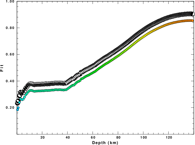
The best fit as a function of depth is given in the following figure:
|
|
Figure 2. Depth sensitivity for waveform mechanism
|
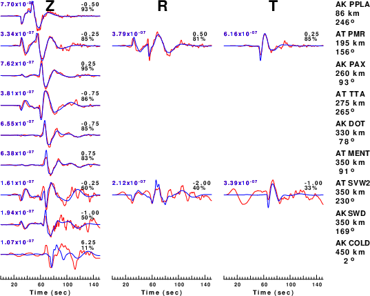
The comparison of the observed and predicted waveforms is given in the next figure. The red traces are the observed and the blue are the predicted.
Each observed-predicted component is plotted to the same scale and peak amplitudes are indicated by the numbers to the left of each trace. A pair of numbers is given in black at the right of each predicted traces. The upper number it the time shift required for maximum correlation between the observed and predicted traces. This time shift is required because the synthetics are not computed at exactly the same distance as the observed, the velocity model used in the predictions may not be perfect and the epicentral parameters may be be off.
A positive time shift indicates that the prediction is too fast and should be delayed to match the observed trace (shift to the right in this figure). A negative value indicates that the prediction is too slow. The lower number gives the percentage of variance reduction to characterize the individual goodness of fit (100% indicates a perfect fit).
The bandpass filter used in the processing and for the display was
cut a -30 a 120
rtr
taper w 0.1
hp c 0.02 n 3
lp c 0.05 n 3
|
|
Figure 3. Waveform comparison for selected depth. Red: observed; Blue - predicted. The time shift with respect to the model prediction is indicated. The percent of fit is also indicated. The time scale is relative to the first trace sample.
|
|
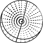
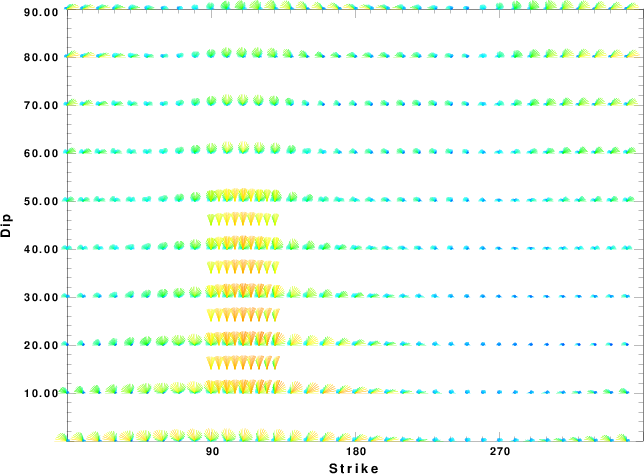
|
Focal mechanism sensitivity at the preferred depth. The red color indicates a very good fit to the waveforms.
Each solution is plotted as a vector at a given value of strike and dip with the angle of the vector representing the rake angle, measured, with respect to the upward vertical (N) in the figure.
|
A check on the assumed source location is possible by looking at the time shifts between the observed and predicted traces. The time shifts for waveform matching arise for several reasons:
- The origin time and epicentral distance are incorrect
- The velocity model used for the inversion is incorrect
- The velocity model used to define the P-arrival time is not the
same as the velocity model used for the waveform inversion
(assuming that the initial trace alignment is based on the
P arrival time)
Assuming only a mislocation, the time shifts are fit to a functional form:
Time_shift = A + B cos Azimuth + C Sin Azimuth
The time shifts for this inversion lead to the next figure:
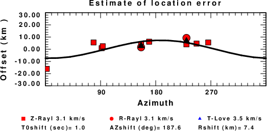
The derived shift in origin time and epicentral coordinates are given at the bottom of the figure.
Velocity Model
The WUS.model used for the waveform synthetic seismograms and for the surface wave eigenfunctions and dispersion is as follows
(The format is in the model96 format of Computer Programs in Seismology).
MODEL.01
Model after     8 iterations
ISOTROPIC
KGS
FLAT EARTH
1-D
CONSTANT VELOCITY
LINE08
LINE09
LINE10
LINE11
      H(KM)   VP(KM/S)   VS(KM/S) RHO(GM/CC)         QP         QS       ETAP       ETAS      FREFP      FREFS
     1.9000     3.4065     2.0089     2.2150  0.302E-02  0.679E-02   0.00       0.00       1.00       1.00
     6.1000     5.5445     3.2953     2.6089  0.349E-02  0.784E-02   0.00       0.00       1.00       1.00
    13.0000     6.2708     3.7396     2.7812  0.212E-02  0.476E-02   0.00       0.00       1.00       1.00
    19.0000     6.4075     3.7680     2.8223  0.111E-02  0.249E-02   0.00       0.00       1.00       1.00
     0.0000     7.9000     4.6200     3.2760  0.164E-10  0.370E-10   0.00       0.00       1.00       1.00
Last Changed Fri Apr 26 08:01:13 PM CDT 2024